Topic 1.2: Defining Limits and Using Limit Notation

The limit

We call the number that the averages close in on a limit. Newton and Leibniz built calculus on speeds like this more than three hundred years ago, but mathematicians argued for a long time about what a speed at an instant really meant. A bishop named George Berkeley mocked the vanishing amounts behind those speeds as the ghosts of departed quantities.

It took mathematicians nearly a hundred more years to pin the idea down. In math we write it in one line, the limit, as h approaches zero, of A of h, equals thirty. The h arrow zero underneath says the input gets closer and closer to zero without ever being zero. The thirty is where the outputs are heading.

If we graph the average A against h, we get a straight line with exactly one point missing, the hole at h equals zero, because that’s the one window that doesn’t exist. Make a guess before I show you. If you demand an average within one meter per second of thirty, how wide can the window be on each side?

This band is that demand. Within one meter per second of thirty, every window narrower than two tenths of a second, on either side, keeps the average inside it. The line drops five for every second of h, so I divide your demand by five. A tenth of a meter per second needs two hundredths of a second, and a hundredth needs two thousandths.

You can never ask for an accuracy I can’t deliver. That’s the meaning of the limit. We can make A of h as close to thirty as we like by taking h close enough to zero, without ever letting h be zero. Let’s make sure the notation reads right, so which sentence says what this limit statement means?

Let’s use A of h to see why the averages approach exactly thirty. Put one plus h into the position formula and multiply out, and you get forty plus forty h, minus five, minus ten h, minus five h squared. That tidies up to thirty-five plus thirty h minus five h squared. Take away the thirty-five meters the car had already covered, and the change in position is thirty h minus five h squared.

Dividing that by h leaves thirty minus five h, and that five is why the line drops five for every second of h. We can cancel the h because we’ve kept h different from zero.

Check it against the table. A tenth of a second gives thirty minus a half, twenty-nine point five, just like the ladder said. As h approaches zero, five h approaches zero, so A of h approaches thirty. That’s why the limit is exactly thirty, and a table could only hint at it.

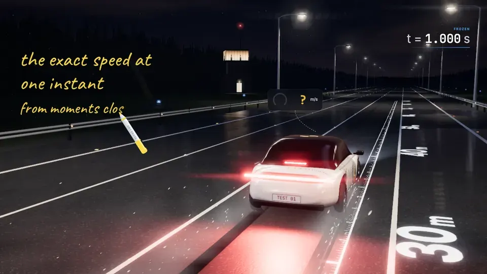
Now we can answer our puzzle. The speed at an instant, its instantaneous rate of change, is the limit of the average speeds around it, and for our car at one second that’s thirty meters per second. We never divided zero by zero, not once. We only ever looked at windows that aren’t zero, and asked where their averages were heading.

The number in the hole

If you took precalc with us, you’ve met this rocket before, frozen one minute after liftoff on Crew Dragon’s first flight to orbit. That was March 2019. Shrinking time windows around this moment made its average climb rate settle on about two hundred seventy-nine and a half meters per second, the same move we just made with the car.

This graph plots the rocket’s average climb rate over a window of width delta, the rocket’s name for our h, against delta itself. Just like the car’s graph, it has nothing at delta equals zero.

From both sides the averages slide toward the same height, though here the two sides aren’t mirror images. Right at zero there’s a hole, because a window of width zero is zero meters in zero seconds all over again.

A of zero is undefined, and yet the limit as delta approaches zero is about two hundred seventy-nine and a half meters per second. Both are true at once, because a limit only ever looks at windows near zero. Let’s play the accuracy game here. Demand an average within one meter per second of the limit, and a window of about three tenths of a second on either side does the job.

Now you set the demand. Pick an accuracy at least as tight as a tenth of a meter per second, then drag the edge of the window until the whole stretch of curve glows green. Whatever accuracy you ask for, a small enough window delivers it.

Real flights don’t come with a formula, so here are the readings from the launch webcast, in kilometers. Using the narrowest interval in the table that contains sixty seconds, estimate the rocket’s climb rate there, in meters per second.

That’s close to the model’s two seventy-nine and a half without matching it. The table’s narrowest window is four seconds wide and the readings are a little noisy, so a table can only give you an estimate. That’s how the AP exam asks it, so pick the narrowest interval around the instant, show your work, and give the units.

Near, not at

If I pull one point out of a line, can the nearby values still tell us where it’s heading? Let’s try it with two x plus one at x equals two, the same kind of picture as our car’s graph. As x gets close to two from either side, the outputs get close to five, so the limit as x approaches two is five, hole or no hole.

It’s the same sentence we wrote for the car, with new letters. The limit of f of x as x approaches c equals R means f of x gets close to R as x gets close to c. Here c is two and R is five. Now let me do something sneaky and define f of two to be nine, so there’s a lone dot floating up here. What do you think happens to the limit?

Nothing happens to it at all, because the limit only cares about inputs near two, never at two. The limit is still five, even though f of two is nine. Sometimes a function already equals its limit. If p of x is just five everywhere, every output already equals five, and the limit as x approaches two is five, the same as p of two.

This graph has a hole and a dot at x equals three, so which statement about this function is true? An AP question might ask whether this limit equals f of three. A full-credit answer has to name both numbers and say where each one comes from. No, because as x approaches three from either side, f of x approaches four, so the limit is four. But f of three is one, and four isn’t one.

You can say every limit four ways, and on the exam you’ll need all of them. In words, as x gets close to three, g of x gets close to seven. In notation, that’s the limit of g of x as x approaches three equals seven. In a table, the inputs creep in toward three from both sides while the outputs creep in toward seven.

On a graph, both sides of the curve close in on the height seven. All four say the same thing. This table gives a function’s values near x equals four, so which statement does it support?

Thirty, at an instant

Let’s go back to our car for one last job. I’ve moved the frozen instant to two seconds into the stop, and the speedometer has gone blank again. This one’s all yours, so squeeze the window in from both sides, find the car’s speed at exactly two seconds, and set it on the dashboard. You’ve found the speed, so now write it down. Which line says what you just found?

There it is on the dashboard, twenty meters per second, and it comes from shrinking the windows until both averages closed in on one number. Back at our first frozen instant, one second in, the promise is kept. Give you a position and a frozen instant, and you can pull out the exact speed by shrinking the windows. You can also write it in one line, the limit as h approaches zero of the average speed equals thirty.

Can change happen at an instant, then? It can, because the instantaneous rate of change is the limit of the average rates of change around it, and Berkeley’s ghosts finally have a proper name. Next time we’ll go hunting on stranger graphs, where the two sides disagree or the function goes wild near the point, and work out when a limit exists at all.