AP Calculus BC Topic 1.3: Estimating Limit Values from Graphs

Topic 1.3 key terms

limit: $\lim_{x\to a} f(x) = L$ means that as $x$ gets close to $a$ from both sides (but never equal to $a$ ), $f(x)$ gets close to $L$ and stays close. The limit never uses the value $f(a)$ .
one-sided limit: The height $f(x)$ approaches as $x$ closes in on $a$ from one side only: from the left ( $x<a$ ), written $\lim_{x\to a^-} f(x)$ , or from the right ( $x>a$ ), written $\lim_{x\to a^+} f(x)$ . The sign describes the inputs, never the outputs.
value at a point: $f(a)$ , what the function actually equals at $x=a$ : the filled dot on a graph, the middle entry of a table. It can equal the limit, differ from it, or not exist at all, and the limit does not depend on it.
does not exist (DNE): A limit does not exist when the outputs never settle on one finite height: the two one-sided limits disagree (a jump), the outputs grow without bound, or the function oscillates without ever settling.
unbounded: Outputs become arbitrarily large in size near $a$ . Write $\lim_{x\to a} f(x)=+\infty$ when both sides grow without bound and $-\infty$ when both fall without bound; this describes how the limit fails, since no finite limit exists. If one side goes to $+\infty$ and the other to $-\infty$ , just say the limit does not exist.
oscillation without settling: Near $a$ the outputs keep returning to separated heights however close $x$ gets, as $\cos(\pi/x)$ swings between $-1$ and $1$ near 0, so they never approach one value and the limit does not exist. (Oscillations that shrink toward one height, like $x\sin(1/x)$ near 0, can still have a limit.)
estimate from a table: Read a table from both ends toward $a$ and see which height both sides close in on. A table suggests a limit; it can never prove one, because it shows only finitely many inputs.

Transcript

1,353 words · 4 parts

The rotor that stopped

This rescue helicopter is about to lift off a cliff, so keep your eyes on the rotor. The whole machine is climbing off the ground, and the blades are just hanging there in the air, perfectly still. There’s no trick editing here. The camera recorded exactly what was in front of it, twenty-five pictures every second.

Now look at the same moment through your own eyes, standing right beside the camera. The rotor is a blur, because it’s really turning five times every second. How can an honest camera show it standing still?

By the end of this lesson, you’ll be able to explain exactly how a camera freezes a spinning rotor, and you’ll catch a graph or a table when it tries the very same trick on you. The secret is that a camera never actually watches anything. It takes snapshots, one every twenty-fifth of a second, and a table of numbers is a set of snapshots too, so that’s where we’ll start.

Where is it heading?

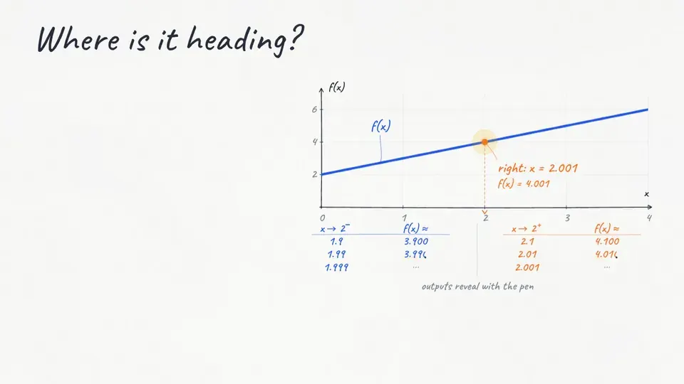
Last lesson you saw that a limit doesn’t care about a hole, or about a dot floating somewhere else. Today we’ll read graphs and tables the way the exam does, one side at a time. Let’s take a few snapshots close to x equals two, first from the left and then from the right.

Start on the left at one point nine, and f gives us three point nine. Move closer, to one point nine nine, and the output moves to three point nine nine. Each extra nine pulls the input toward two and the output toward four. Now start just above two, at two point one, where the output is four point one.

As the inputs come in through two point zero one and two point zero zero one, the outputs come down toward four, so we land on the same height from this side too. Both sides are closing in on the same height, four, and that’s exactly what we mean when we write that the limit of f of x, as x approaches two, equals four.

Here f of two is also four, so all three answers agree, and that’s the ordinary case where nothing strange happens at all. Whenever you read a graph near a point, there are really three separate questions to ask, where it heads from the left, where it heads from the right, and what’s actually sitting at the point. The limit only cares about the first two, and the dot only answers the third, so always keep them in separate boxes.

On this new curve, both sides come down onto four from above. That tells you that from the left describes the inputs, the x’s smaller than two, never the direction the outputs come from.

Two sides of a boom

In 1973, the United States banned civilian planes from flying faster than sound over the country without special permission, and the reason was the noise they drag along behind them. Here it comes, and listen for two bangs, not one. A microphone on the ground records the air pressure, and this is the model engineers use for what it hears. The pressure sits at normal, jumps up by about ninety-three pascals, slides down below normal, and jumps back.

Each of those jumps is one of the bangs you heard, because your ear hears a sudden jump in pressure as a boom. A sonic boom is really a jump in a graph. In real air the jump takes a few thousandths of a second, far too quick for your ear, so the model treats it as one instant.

Let’s call the pressure p, call the instant the first bang arrives t equals zero, and sneak up on it from the left, from the moments just before the boom. The whole way in, the pressure stays at zero above normal. Now you try it. Drag the probe in toward the jump from the right side, and watch what the pressure reading settles on.

We write each side with a little sign up top, minus for the times below zero and plus for the times above. The limit as t approaches zero from the left is zero, and from the right it’s about ninety-three. The two sides head for different heights, zero and ninety-three, so there’s no single height the pressure is heading for, and in this model the two-sided limit doesn’t exist.

This is NASA’s X-59. Its whole shape, that ridiculous needle nose included, is there to spread out its shock waves and soften the sharp pressure change that reaches the ground. If it works the way NASA predicts, the jump becomes a gentle rise, and the boom softens into a thump.

In our model of that gentle rise, the two sides agree at every instant, so the limit exists everywhere. NASA built an entire airplane to soften that sudden jump into a gentle rise, and on our graphs, that’s exactly the difference between a limit that fails and one that exists. Now you get to design the jet. Stretch its nose until the jump in the pressure trace disappears.

Let’s put the same idea on the board with friendlier numbers, a function B that heads to four from the left, heads to six from the right, and has its dot at five. Written side by side, the limit from the left is four, the limit from the right is six, and B of two is five. It’s tempting to split the difference and call the limit five, because the dot sits right there in the middle, but neither side ever gets anywhere near five.

When an exam question says justify, a grader wants both one-sided limits and the reason in one sentence, so let’s write it the way that earns the point. Because the limit from the left is four and the limit from the right is six, and those aren’t equal, the limit of B of x as x approaches two does not exist.

Read it like the exam

Here’s the kind of graph the AP exam loves, with a little bit of everything packed into one picture, and we’re going to read it exactly the way a grader would. At x equals negative one there’s a hole. From the left the curve heads to two, and from the right it also heads to two, so the limit is two, even though g of negative one doesn’t exist.

At x equals one, coming from the left the curve climbs toward the open circle at three, and coming from the right it slides down onto the filled dot at one. That makes the left-hand limit three and the right-hand limit one, so the two-sided limit doesn’t exist. The value g of one is one, because the filled dot tells you where the function actually lives at that point.

Let’s do the next one together. Look at x equals three, where the curve has a hole and a lonely filled dot floats above it. What’s the limit of g of x as x approaches three?

Now try one on your own. Exactly one of these four limits does not exist, and I want you to find it. There’s one more place on this graph, at x equals negative three, where the curve shoots up forever on the left and plunges down forever on the right.

If you’ve seen Mean Girls, this is the limit behind the last question of the big math competition. You don’t need to work that formula out, because the graph tells the whole story. Lindsay Lohan’s character looks at it and says the limit does not exist, and she’s completely right, because one side runs up forever and the other runs down forever.

When both sides run up forever, like one over x squared at zero, we write that the limit equals infinity. That infinity describes how the limit fails, because there’s no number the outputs ever settle on. A limit can fail to exist in three ways. The two sides can disagree, the outputs can grow without bound, or the function can swing forever without settling, and that third one is where our frozen rotor comes back in.

Topic 1.3: Estimating Limit Values from Graphs