
The ten points, and how many students earned each
The question has had the same shape on both exams in the current format, 2025 and 2026, and in the sample question in the course framework. Parts A and B are the design. Parts C and D are the analysis, built on a related but different experiment with real data. The course framework suggests 25 to 30 minutes for the whole question.
| Stage | Points in 2025 and 2026 | 2025 mean points | What to check in your answer |
|---|---|---|---|
| Measurements and procedure | 2 | 1.43 | Name measurable quantities and a specific way to reduce uncertainty. |
| Proposed graph and its interpretation | 2 | 0.64 | Choose a useful relationship and explain how it reveals the unknown. |
| Plotting and fitting the supplied data | 4 | 2.30 | Use a labelled scale, consistent data transformations and a fit that follows the trend. |
| Extracting the unknown | 2 | 0.56 | Connect the fitted relationship to the quantity being measured. |
The procedure is not where students fall down: about 7 in 10 earned each of the first two points. The losses cluster in B2, D1 and D2, and all three ask for the same move, connecting a slope to the quantity you were sent to find. The next-biggest loss is C2, an axis label with its unit, which is the easiest point on the page to keep.
Parts A and B: designing the experiment
The course framework sets the rules for a design. Change one quantity, measure how one other quantity responds, use equipment a high school lab would have, and say how you would analyze the data, usually with a graph.
Start from the physics
Before you write a single step, write the equation that connects what you can change to what you want to find. It tells you what to vary, what to measure and what the slope will mean, and it keeps you from measuring things you don’t need. In 2025 that equation was a torque balance about the pivot. In 2026 it was energy: the block’s at the top of the ramp, all of it removed by friction over the sliding distance.
Correct 2025 answers set the torque from the spring scale equal to the torque from the hanging block. A common wrong start was to set the spring scale’s reading equal to the block’s weight, wherever the block hung.
Know what each instrument measures
The course framework lists the lab equipment you should know, and it is specific about what each piece actually measures. Exam questions lean on those details.
| Instrument | What it measures | Keep in mind |
|---|---|---|
| Meterstick | Length: heights, distances, stretches | Say which distance you mean: “from the pivot to the block,” not “the distance.” |
| Balance or scale | Mass | Some questions take it away. In 2025 there was no way to weigh the block, so its mass had to come from a slope. |
| Stopwatch or phone timer | Time | For periodic motion, time several complete cycles together and divide, so your reaction time matters less. |
| Spring scale or force sensor | The force on its hook | It does not measure torque. It reads a hanging object’s weight only when the object hangs straight from it and isn’t accelerating. |
| Photogate | How long its light beam is blocked; with the object’s length, a computer turns that into speed | One gate gives the speed at that spot, two gates the time between them. It can’t tell which way the object moves. |
| Motion sensor | The time for an ultrasonic echo to come back | Software turns those times into position, velocity and acceleration. |
| Pressure sensor | Pressure | The course framework’s sample question uses one, with a meterstick, to find a liquid’s density. |
Write steps a classmate could follow
- Name every quantity you measure and the instrument you measure it with.
- Say what you change, over what range, and what stays the same. Five or more different values give you a line worth drawing.
- Say what you record at each setting.
- Leave out “gather the equipment” and “record the data in a neat table.” The 2025 Chief Reader asked teachers to have students edit those lines out. They earn nothing and cost time.
Reduce the uncertainty with one specific action
Both rubrics accepted either of two moves: repeat the measurement at the same setting and average, or take measurements at several different settings. Write it as an action tied to a quantity, such as “repeat each release height three times and average the sliding distances.” “Be careful” is not a method.
This point is judged on its own. In the 2025 sample responses College Board published, one answer lost it by taking a single force reading at a single hole, and another earned it with a procedure that was wrong in other ways, because it said to repeat the measurement three to five times.
Part B: name the graph, then say what the slope equals
B1 asks which two quantities you would graph. Either one can go on either axis; the 2025 and 2026 rubrics accepted any arrangement with the right relationship between them. B2 is the point only 1 in 5 students earned in 2025: write the slope as an expression, then solve it for the unknown.
The biggest problem the Chief Reader saw in part B was two distances with similar names: from the pivot to the block, and from the pivot to the spring scale. Give each one its own symbol and say what it is.
Linearization: making the graph a straight line
A curve is hard to read by hand. A straight line has a slope you can measure from two points, and on both released versions of this question the analysis was built around that slope. Linearizing means choosing what to plot so the relationship comes out straight.
The method in four steps
- Write the equation that connects the quantities, from the reference sheet or from your own derivation.
- Find the two quantities that change from trial to trial: the one you set and the one you measure. Everything else in the equation is a constant, including the unknown you want.
- Rearrange into the form , where and can be any expression of your two changing quantities, such as , , or .
- Read the slope off as a group of constants, and solve that for the unknown.
The 2025 Chief Reader offered a shortcut for fractions. If the relationship can be written as a fraction, graph the numerator against the denominator, and the slope is the quantity left over. Density is the simplest case: , so graph against and the slope is .
Two real examples
2025: . The quantities that change are and ; , and the are constants. Rewrite it as : plot against , and the slope is .
2026: looks harder than it is. Only and change between trials, and , and stay fixed. So , , and the whole bracket is the slope, . All of the difficulty is in the algebra afterward.
| d (m) | v (m/s) | v² (m²/s²) |
|---|---|---|
| 0.15 | 0.43 | 0.185 |
| 0.25 | 0.56 | 0.314 |
| 0.35 | 0.65 | 0.423 |
| 0.45 | 0.75 | 0.563 |
| 0.55 | 0.82 | 0.672 |
A best-fit line through these practice points has a slope of about 1.22 m/s². Using m/s², , so . These practice values do not use the 2026 scoring guideline’s numerical range.
The reference sheet’s equations, linearized for the lab
The 2025 Chief Reader’s advice to teachers was to take every equation on the reference sheet and practice deciding what to measure and plot to get a straight line, and what that line could tell you. Here is that exercise done for 23 setups a school lab can run, each built on equations from the sheet. To use it as practice, cover the last two columns and fill them in yourself.
| Equation on the sheet | You change | You measure | Plot | Slope |
|---|---|---|---|---|
| , released from rest | Distance traveled | Time, with a stopwatch | against | |
| , released from rest | Distance to a photogate | Speed at the gate | against | |
| Time | Velocity, from a motion sensor | against | (intercept: ) | |
| , a cart pulled by a hanging mass | The hanging weight, moving masses from the cart to the hanger so the total stays fixed | Acceleration | against | |
| The hanging weight | The stretch | against | ||
| , block pulled at constant speed | The normal force, by stacking masses on the block | The pulling force, on a spring scale | against | |
| , with , a mass on a string circling on a level, frictionless table | Speed around the circle | The string force, on a force sensor | against |
| Equation on the sheet | You change | You measure | Plot | Slope |
|---|---|---|---|---|
| and , no friction | Drop height | Speed at the bottom | against | |
| and , a block descending a frictionless ramp, then stopping on a rough horizontal surface (2026) | Release height | Sliding distance | against | |
| and , a spring launcher | Compression | Launch speed | against | |
| The impulse, from the area under a force sensor’s force-time graph | The change in velocity | against | ||
| , a beam balanced on a pivot (2025) | The hanging block’s distance from the pivot | The balancing force , applied at a fixed distance | against | |
| Time | Angular speed , from a photogate on a pulley or a video | against | (intercept: ) | |
| , from rest | Time | The angle turned | against | |
| The torque , from a string pulled with a force sensor | Angular acceleration | against | ||
| , two equal masses slid along a rod | Each mass’s distance from the axis | Rotational inertia , found as | against | (intercept: the rod’s own ) |
| Equation on the sheet | You change | You measure | Plot | Slope |
|---|---|---|---|---|
| The hanging mass | The period | against | ||
| , small swings | The length | The period | against | |
| Sample size | Mass and volume | against | ||
| Depth | Pressure , with a pressure sensor | against | (intercept: ) | |
| The submerged volume | The buoyant force: the scale reading in air minus the reading underwater | against | ||
| , a fixed flow rate | The nozzle area | The exit speed | against | The volume flow rate |
| , water leaving a hole in an open tank | The hole’s depth below the surface | The exit speed | against |
Parts C and D: the graph and the slope
Label the axis with a quantity and its unit
Write both, as in “ (m²/s²)” or “Force (N)”. In 2025 this was the most-missed graphing point: 39% earned it, and the Chief Reader said many students wrote only a label or only a unit. If the quantity has no unit, such as , leave the unit off. A 2025 sample response that did that for a unitless quantity still earned the point.
Choose an even scale that fills the grid
Use equal steps between gridlines, starting from a round number, and stretch the scale so the data cover most of the grid. Nearly every student in 2025 managed an even scale. Spreading the points out makes the slope easier to read accurately.
Calculate first, then plot
Work out every plotted value before you touch the grid, in the table the booklet gives you (in 2026 that table was scratch space and was not scored). Doing the squaring and the reciprocals in the table, not in your head while plotting, keeps points from landing in the wrong place.
Draw one straight line
Use a ruler. The line should follow the trend, with points scattered on both sides. It doesn’t have to pass through any particular point, or through the origin. The Chief Reader saw students join the dots instead, which is not a best-fit line. If an earlier mistake made your points curve, a smooth curve that follows them still earns the line point.
Take the slope from your line, then use it
Pick two points on the line itself, far apart, and read them off the grid. Show the subtraction and the units. Then do the step most students skipped in 2025: write the slope as an expression from the equation and solve it for the unknown. That one line was D1, earned by 28%.
Worked example: 2025 Question 3
This is the question with the most data behind it, because the 2025 Chief Reader report gives the average for each of its ten points. Read the full prompt and figures in College Board’s 2025 questions (PDF). The response was written for this page; check it with the 2025 scoring guidelines.
Open the 2025 released question, Question 3 for the prompt and diagrams. Our worked solution follows; the official scoring guidelines give the complete rubric.
A: Hang the block from the 60 cm hole, 0.10 m from the pivot. Pull down on the spring scale at the left end, 0.50 m from the pivot, until the meterstick is level, and record the force it reads. Repeat with the block at 70, 80 and 90 cm (0.20, 0.30 and 0.40 m from the pivot). Take three readings at each hole and average them.
B: With the stick level, the torques about the pivot balance: , where is the distance from the pivot to the block. So . Graph on the vertical axis against . The slope is , so .
C(i): Vertical axis: (N).
C(ii): [Values worked out first: = 2.67, 1.94, 1.70, 1.41 and 1.02, with = 21, 17, 13, 12 and 8 N. Vertical axis labeled “ (N)” from 0 to 25 N in steps of 5 N. Five points plotted.]
C(iii): [One straight line drawn with a ruler through the middle of the points. It passes through (0.50, 4.3 N) and (2.50, 20.1 N).]
D: Slope from two points on my line: . Since , the slope is , so .
Why it works
- Part A needs the block hanging on the meterstick and a force reading taken with it there. Hanging the block from the spring scale was ruled out by the question, so its mass has to come out of the meterstick experiment.
- Naming the two distances separately, “from the pivot to the block” and “0.50 m from the pivot to the spring scale,” avoids the mix-up the Chief Reader called the biggest challenge in part B.
- The slope comes out in newtons because the horizontal quantity, , has no unit.
- The line misses the origin by a little, and that is fine. The slope is what you use, and it came from the line, not from two data points.
A weaker response to the same question
Here is the kind of answer that scores well below the 2025 average. It was written for this page, and its mistakes are the ones the Chief Reader report and the published sample responses describe.
A: Gather a meterstick, a spring scale and the block. Hang the block from the spring scale to find its weight. Record the data in a neat table.
B: Graph the force against the mass of the block. The slope is .
C(i):
C(ii): [Vertical axis labeled “Tension” with no unit, scale 0 to 25 in steps of 5, five points plotted correctly.]
C(iii): [Short straight segments joining each point to the next.]
D: Slope . Slope , so .
Why it works
- The procedure tries to weigh the block directly, which the apparatus does not permit, and never repeats a measurement. There is no usable graph of force against a mass that cannot be varied or measured.
- The analysis chooses the right vertical quantity and places the data correctly, but omits the force unit and joins successive points. Those are separate mistakes.
- The slope must be linked to the apparatus: here it is , not . Using the latter produces 0.81 kg instead of about 0.97 kg. The numerical agreement between a two-data-point slope and a fitted slope here is accidental.
- Under the linked 2025 rubric, only the chosen vertical quantity and the plotted points earn credit: 2 of 10.
Three of the eight lost points (A1, B1 and B2) trace back to one decision in the first sentence: treating this as a problem about the spring scale instead of about torque. The other five come from habits covered above: repeated readings, a unit on the axis, a ruler line, and the slope written out before the numbers.
Mistakes the 2025 Chief Reader saw
- Treating the spring scale’s reading as the block’s weight, wherever the block hung. The scale was balancing a torque, so its reading depended on where the block was.
- Saying a spring scale measures torque. It measures force. Torque comes from multiplying a force by a distance.
- Mixing up two distances with similar names, such as pivot-to-block and pivot-to-scale.
- An axis with a label and no unit, or a unit and no label.
- Plotting a reciprocal that bends the line, such as against .
- Joining the dots instead of drawing one best-fit line.
- Calculating a slope and stopping, without saying how it relates to the unknown.
- Padding the procedure with steps like “gather equipment” that earn nothing.
Practice
Three questions in this format are public. The two exam questions are 2025 Question 3 (scoring guidelines) and 2026 Question 3 (scoring guidelines). The third is the sample in the course and exam description, which finds a liquid’s density with a pressure sensor and then from the speed of water leaving holes in a tank.
Give yourself 25 minutes for each, write a full answer, then score it one point at a time against the scoring guidelines. After that, cover the last two columns of the linearization tables above and fill them in from memory.
The lessons behind the most common lab setups:
 Topic 1.325 minRepresenting Motion
 Topic 2.722 minKinetic and Static Friction
 Topic 2.825 minSpring Forces
 Topic 5.327 minTorque
 Topic 5.526 minRotational Equilibrium and Newton's First Law in Rotational Form
 Topic 7.221 minFrequency and Period of SHM
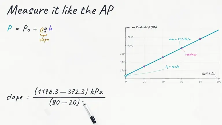 Topic 8.231 minPressure
 Topic 8.330 minFluids and Newton's Laws
For the other three free-response questions, see the AP Physics 1 FRQ guide. For every equation and idea in the course on a few pages, use the AP Physics 1 cheat sheets.
Sources
- AP Physics 1: Algebra-Based Course and Exam Description: the Experimental Design and Analysis question, lab equipment, sample question and scoring (PDF)
- 2025 AP Physics 1 Free-Response Questions, Question 3 (PDF)
- 2025 AP Physics 1 Scoring Guidelines, Question 3 (PDF)
- 2025 AP Physics 1 Chief Reader Report: Question 3 point averages, errors and advice (PDF)
- 2025 AP Physics 1 Question 3 sample responses and scoring commentary (PDF)
- 2026 AP Physics 1 Free-Response Questions, Question 3 (PDF)
- 2026 AP Physics 1 Scoring Guidelines, Question 3 (PDF)
- AP Physics 1 reference sheet, mechanics and fluids (PDF)
- AP Physics 1 past exam questions, AP Central