
Topic 5.3 key terms
- increasing on an interval
- f is increasing on an interval if, for any a < b in it, f(a) < f(b). If f′(x) > 0 for every x in an interval, f is increasing there.
- decreasing on an interval
- f is decreasing on an interval if, for any a < b in it, f(a) > f(b). If f′(x) < 0 for every x in an interval, f is decreasing there.
- critical point
- An input c in the domain of f where f′(c) = 0 or f′(c) does not exist. Critical points are the only candidates for relative extrema; not every critical point is one.
- relative (local) maximum
- f has a relative maximum at c if f(c) is greater than or equal to every value of f for x near c.
- relative (local) minimum
- f has a relative minimum at c if f(c) is less than or equal to every value of f for x near c.
- First Derivative Test
- For f continuous at a critical point c: if f′ changes from positive to negative at c, f has a relative maximum at c; from negative to positive, a relative minimum; if f′ is positive on both sides of c (or negative on both sides), f has no relative extremum at c.
- sign chart
- A number line for f′ cut at its zeros, undefined points and domain gaps, with the sign of f′ on each piece from one test value. It finds the answer; the written reason about f′ justifies it.
- location vs value
- A relative maximum happens AT x = c (the location); its value is f(c). For f(x) = x³ − 6x² + 9x + 1 the relative maximum is at x = 1 and its value is f(1) = 5.
Transcript
672 words · 2 parts
Christmas Eve, 2024
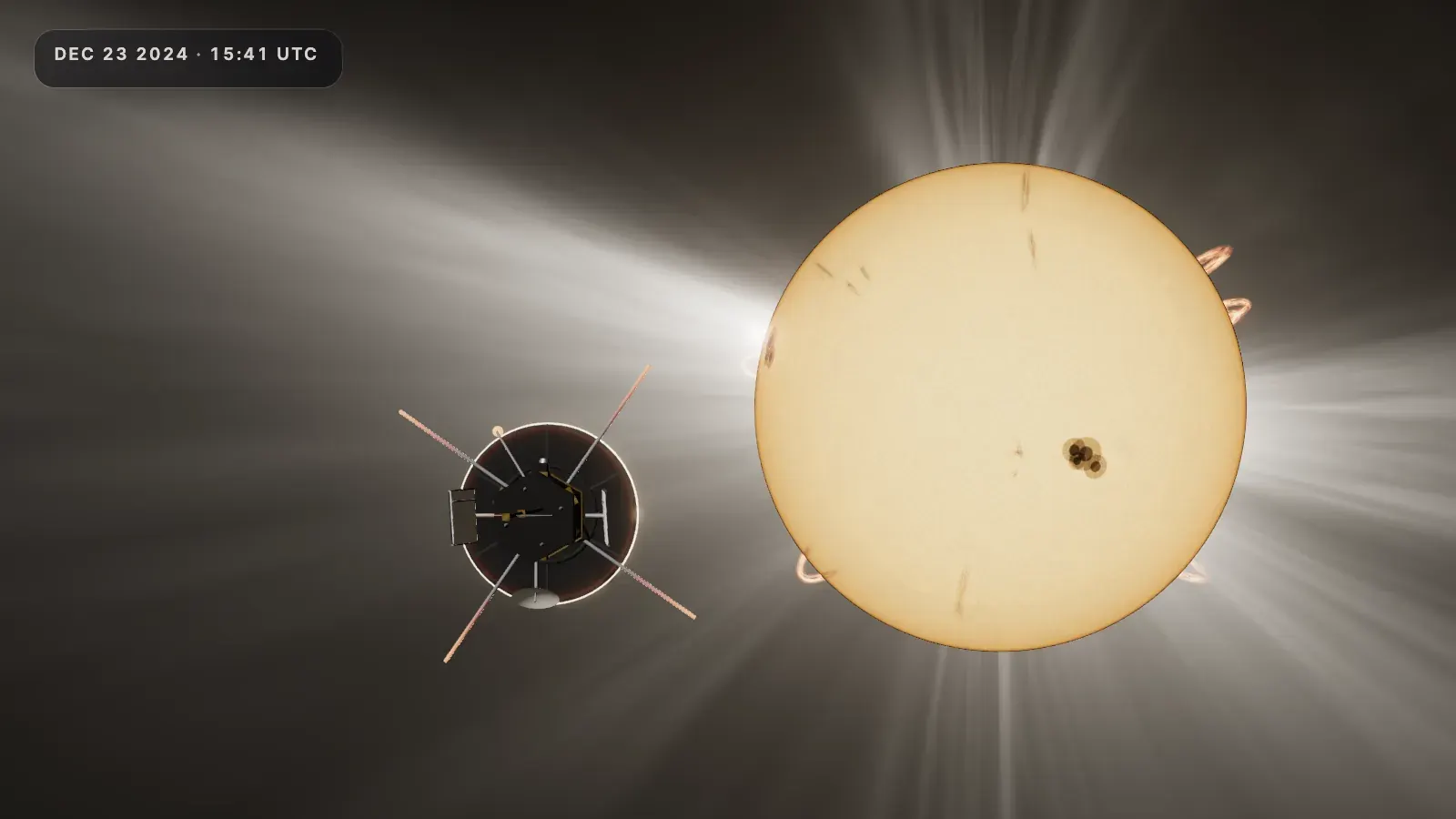
This is Parker Solar Probe, a spacecraft about the size of a small car, and on Christmas Eve 2024 it flew closer to the Sun than anything people have ever built. It passed just three point eight million miles above the Sun’s surface. That sounds far until you shrink it down, because if the Earth and the Sun were one meter apart, Parker would be about four centimeters from the Sun.
It was moving at about four hundred thirty thousand miles an hour, roughly a hundred ninety kilometers every second. That’s fast enough to fly from Washington to Tokyo in under a minute, and no human-made object had ever moved that fast. Now watch two numbers at the very moment it’s closest. Its speed is the highest it gets anywhere on its orbit, and at that exact same instant, the rate at which its distance from the Sun is changing is zero.
How can something moving that fast have a distance that isn’t changing at all? If we watch whether the distance shrinks or grows on either side of that zero, we can tell exactly what kind of moment this is.
By the end of this lesson, you’ll be able to find the exact moment this probe was closest to the Sun using nothing but that rate, and prove it with the one sentence that earns full credit on the AP exam. So let’s start with the simplest question you can ask about any rate, which is whether it’s positive or negative.
Shrinking or growing
Let’s call the probe’s distance from the Sun r, and since that distance changes as time goes by, it’s a function of time, r of t. On the way in, the distance keeps shrinking, so its rate of change, r prime, is negative, and you can see the arrow at the probe pointing straight at the Sun.
Right at the closest point, the probe is moving straight sideways, across the line to the Sun, so for that one instant it gets neither closer to the Sun nor farther away. That’s how all that speed can come with a rate of zero. Then it climbs back out, the distance grows, and r prime turns positive, until out at the far end it shrinks back to zero and the fall begins again.
And the probe has been drawing its own graph the whole time. While r prime is below zero, the graph of r runs downhill, and while r prime is above zero, it runs uphill. At this scale the bottom of that dip looks almost like a corner, because the probe whips around the Sun in about a day, but zoom in and it’s a smooth, rounded valley, and r prime slides right through zero.
Twenty days after its closest pass, the probe has slowed way down, from about one hundred ninety kilometers a second to about twenty-eight, and it’s still slowing. So right now, what’s the sign of r prime?
Let’s take this onto the board with a function we can actually write down, f of x equals x cubed minus six x squared plus nine x plus one. Underneath it is its derivative, f prime, lined up so that every x has its own spot on both graphs. Watch the tangent line on f as I slide along. Wherever f prime sits above its axis, the tangent tilts up and f climbs, and wherever f prime drops below the axis, f runs downhill.
So if f prime is positive on an interval, then f is increasing on that interval. In the same way, if f prime is negative on an interval, f is decreasing there. Notice it’s only the sign of f prime that matters, not the sign of f. Down here f itself is negative, but f prime is positive, so f is still increasing.
Now let’s hide f and keep only its derivative, which is exactly how the AP exam likes to ask it. Using just the graph of f prime, on which interval is f decreasing?