Topic 10.11: Finding Taylor Polynomial Approximations of Functions

Thread the hoop

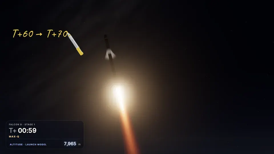
You’ve met this rocket before. In Unit 4 we tried to forecast where it would be ten seconds after T plus sixty, using nothing but its tangent line. Let’s hang a hoop of light where that forecast says the rocket will be at exactly T plus seventy, and see if it keeps the appointment. At T plus seventy it’s three hundred forty-six meters above the hoop, way too high.

Let’s rewind and give the forecast one more number from that same instant, how fast the climb rate is changing. We brought the forecast much closer, but at seventy seconds the rocket is still about twenty-two meters above it. Rewind once more, and add one more number. It threads the hoop, sixty-five centimeters off, after more than three kilometers of climbing.

Every one of those forecasts came from one single instant. By the end of this lesson, you’ll build that last forecast yourself. Then you’ll do the same for any smooth function, using what it’s doing at one point to predict its values nearby. What did the third forecast know that the first one didn’t? Let’s start with the one that missed.

What a straight line knows

Here’s that forecast as a graph of altitude against time. The curve is the rocket’s altitude model from precalc, which came from the real flight’s readings, and the forecast is its tangent line at T plus sixty.

It’s h of sixty plus h prime of sixty times t minus sixty, so it gets two things exactly right at T plus sixty, the height and the slope. From now on we’ll call it T one, the first-degree Taylor polynomial. But the rocket is speeding up, so the curve bends upward, away from the line, and the line has no way of knowing that.

Bend it

To teach a forecast how to bend, let’s practice on a friendlier curve, cosine of x near zero, in radians. At zero, cosine sits on top of the hill at height one with a slope of zero, so its tangent line is the flat line y equals one. That line is a great forecast right at zero and a bad one a unit away.

Let’s give the line a bend by adding c times x squared, where we get to choose c. That doesn’t spoil what we already had, because at zero, c x squared adds nothing to the height, and its derivative, two c x, adds nothing to the slope. All c changes is the bend. A positive c curls the ends the wrong way, and c equals negative one bends down too hard.

Now you find it. Drag c until the parabola hugs cosine near zero as tightly as you can. The tangent line matched the height and the slope. The new idea is to match one more derivative, the second derivative, which measures the bend.

Two derivatives of c x squared give two c, and cosine’s second derivative at zero is negative cosine of zero, negative one. Two c equals negative one, so c is negative one half, exactly what you found with the slider. That half isn’t decoration. Differentiating x squared twice leaves a two behind, and we have to divide it back out.

That makes the second-degree Taylor polynomial for cosine at zero one minus x squared over two. At one half it gives zero point eight seven five, and the true value is about zero point eight seven seven six, within three thousandths. The same matching works at any center a if we measure distance from a. That’s why we write powers of x minus a, just like t minus sixty for the rocket.

The height gives c zero equals f of a. The slope gives c one equals f prime of a. And the bend gives c two equals f double prime of a, over two. For the rocket, that’s half its vertical acceleration, the same one half as in one half a t squared from physics.

Where the factorials come from

To match a third derivative, let’s add c three times x minus a cubed and see what it does at the center. Each derivative brings the exponent down in front. Take one derivative, and the three comes down. Take another, and the two comes down. One more, and the one comes down, which leaves three times two times one, times c three.

At x equals a, the first three are all zero, so this term leaves the height, the slope and the bend alone. It only changes the third derivative, which is six c three. Matching f triple prime of a gives c three equals f triple prime of a over six, and six is three factorial.

Let’s try a fourth-degree term, c four times x minus a to the fourth, and differentiate it four times to see what number survives. What number should we divide the fourth derivative by to get c four?

The coefficient of x minus a to the n is the nth derivative at a, divided by n factorial. That’s the whole recipe. Add the terms up to whatever degree you want, and you have the nth-degree Taylor polynomial for f centered at a, or about x equals a, as the exam says it. It matches f’s value and its first n derivatives at the center, and it stops after the term of degree n. With the center at zero, people call it a Maclaurin polynomial.

Let’s run the recipe on cosine, centered at zero, which makes this one a Maclaurin polynomial. Its derivatives at zero cycle through one, zero, negative one, zero, one. If we raise this polynomial’s degree from two to three, what happens to its graph?

At one half, T four and cosine both round to zero point eight seven seven six. T two was off by about three thousandths, so one more term cut the error more than a hundredfold.

Thread it yourself

Back to the rocket. At T plus sixty we measured four numbers, its height, its climb rate, its acceleration, and how fast the acceleration changes. Engineers call that last one jerk, and those last two are what the third forecast knew that the first one didn’t. Our center is sixty, so each derivative goes over its factorial and multiplies the matching power of t minus sixty. Every term comes out in meters, because each derivative has as many per-seconds as its power of t minus sixty has seconds.

At T plus seventy, t minus sixty is ten seconds, and the first two terms give eight thousand ninety-one plus two thousand seven hundred ninety-five, the line that missed. How many meters does the third term, the bend, add to the forecast at T plus seventy? Round to the nearest meter.

The jerk term adds about twenty-one and a half meters, so the cubic forecast is about eleven thousand two hundred thirty-one and a half meters. That’s less than a meter below the launch model’s true altitude.

Notice how fast the terms shrink, from thousands to hundreds to about twenty, which is what you want to see close to the center. Let’s take your forecast back out to the launch, and this time you build it.

All four numbers from T plus sixty are in, but the divisors are up to you. Choose what to divide each derivative by, fly it, and thread the hoop at T plus seventy.

How far can a forecast see?

Let’s push our luck and move the hoop out to T plus eighty. The same cubic forecast now misses by about nine meters. At T plus one hundred it misses by about ninety-six meters. We built this polynomial entirely from what happens at the center, so it’s at its best near the center and usually drifts as you go farther.

Back on cosine, watch what happens as the degree keeps climbing. Each new even power keeps the hug going a little farther out, and by degree sixteen it follows cosine across almost the whole window. In many cases, as the degree goes up, the polynomials close in on the function over some interval.

Here’s the natural log of one plus x, with its second-degree polynomial and a probe at x equals one and a half. If we keep raising the degree, what happens to the forecast at the probe?

More terms don’t always help, and exactly where they stop helping is a story for a later lesson. For the rocket we only measured four numbers, so we can’t add terms, but we can measure at a better moment, closer to the hoop. Moving the hoop asks the same polynomial about a different time, but moving the measurement point builds a brand-new polynomial, with four new numbers on the card.

Now the hoop sits out at T plus ninety, and the forecast stays cubic. Measure as early as you can and still thread it, because every second earlier is more warning.

One more term for the Earth

In Unit 4 you found that the sea falls below a flat beam by about x squared over two R. Here x is the distance along the beam, and R is the Earth’s radius. That parabola was a Taylor polynomial all along.

On a sphere, the drop is R minus the square root of R squared minus x squared. Unit 4 gave us its slope, x over that square root. At the touch point, both are zero. That’s why the beam lies flat.

One more derivative. The product rule gives two pieces. The second piece has an x in front, so at zero it’s gone. The first piece leaves one over the square root of R squared, and that’s one over R.

Divide that by two factorial and you get x squared over two R, the same parabola you found with L’Hospital’s rule, this time from two derivatives instead of a limit. A thousand kilometers out, though, the parabola peels away from the sea by almost five hundred meters, so let’s add the next term.

The drop is the same on both sides of the touch point, just like cosine, so its Taylor polynomial only has even powers. There’s no x cubed term, and the next one that matters is x to the fourth.

The fourth derivative of the drop at zero turns out to be three over R cubed. What’s the coefficient of x to the fourth in the fourth-degree Taylor polynomial?

Watch the new curve at a thousand kilometers. The x to the fourth term adds almost half a kilometer, and the forecast lands about six meters from the sea.

On the exam

Here’s how this shows up on the AP exam. You get derivative values at one point, here x equals two, and they ask for a Taylor polynomial and an estimate. Which of these is the third-degree Taylor polynomial for f about x equals two?

Three mistakes cost points on exactly this question. The first is powers of x when the center isn’t zero, and the second is a plus dot dot dot on a polynomial that should stop. The third is leaving a coefficient like f double prime of two over two factorial instead of working it out. Now use it to approximate f of two point one, to three decimal places.

Sometimes the exam hides the derivatives in a differential equation, like y prime equals x plus y squared, with y equal to one when x is zero. Then y prime at zero is zero plus one squared, which is one. Differentiate again, keeping y a function of x, so y squared gives two y y prime. At zero that’s one plus two times one times one, which is three, so T two is one plus x, plus three over two factorial times x squared, and that’s three halves x squared.

One more exam move runs the recipe backward. The second-degree Taylor polynomial for g about x equals one is four minus three times x minus one squared. The question asks what g is doing at x equals one, and it wants a justification. Before we justify anything, make the call. What does g have at x equals one?

The sentence a grader wants names both facts and the test. G prime of one is zero and g double prime of one is negative six, less than zero, so by the Second Derivative Test, g has a relative maximum at x equals one.

The forecast, kept

Back where we started, every derivative we matched at T plus sixty made the forecast better. The recipe told us exactly how to use each one, the nth derivative over n factorial, times t minus sixty to the n.

It’s best near the center, and farther out you need more terms or a closer measurement. On the exam, write powers of x minus a, divide by the factorial, and stop at the degree they ask for.

You built the forecast that threads the hoop from one single instant of this rocket’s flight. Now you can do the same for any smooth function, using its derivatives at one point to predict its values nearby.

We only knew it was sixty-five centimeters off because we had the true altitude to compare with. How could you know how far off a forecast might be without the answer? That’s the next lesson.