Topic 1.1: Introducing Calculus: Can Change Occur at an Instant?

Ninety to zero

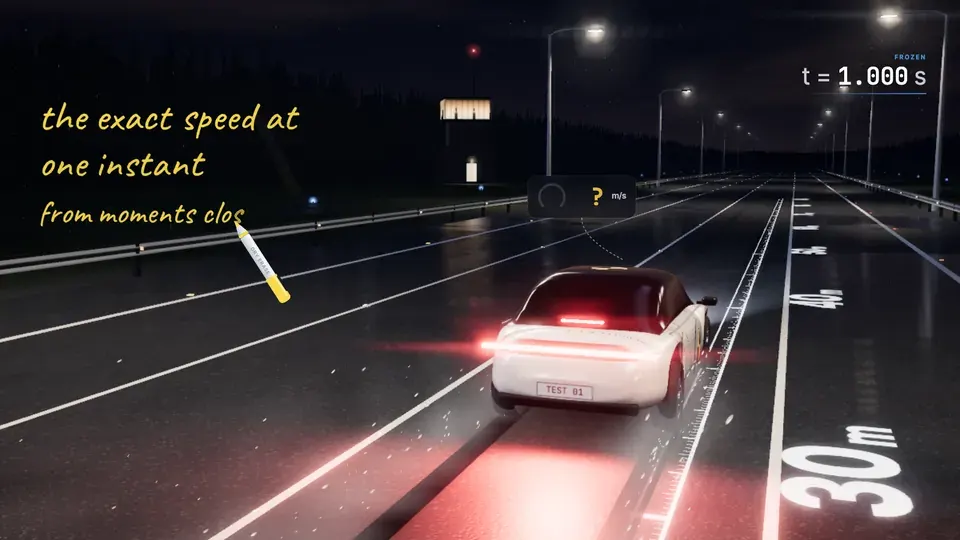
It’s two in the morning on a closed test track, and that pair of headlights way down the road is a test car. It’s coming at us at forty meters per second, about ninety miles an hour.

Right at that white line, the driver stands on the brake pedal as hard as the tires can take it. Let’s freeze time exactly one second after the brakes went on, and the speedometer, frozen along with everything else, says thirty meters per second. That thirty bothers me a little, because a speed is a distance divided by a time, and in one single frozen instant, no time goes by at all.

In zero seconds the car covers zero meters, so the only division we can do right at this instant is zero over zero. Zero divided by zero isn’t a number at all, so what is that thirty actually measuring?

People puzzled over moments like this one for more than two thousand years, and the idea that finally settles it is the idea all of calculus is built on. By the end of this lesson, you’ll be able to take one frozen instant like this and pull out the car’s exact speed. You’ll do it by looking at where the car is at moments closer and closer to this one, before and after.

You’ll also be able to write that answer in a single line, in the notation every calculus course uses for it. Let’s start with the one kind of speed nobody argues about, an average.

Before and after

When we froze it, our car was thirty-five meters past the white line, one second after the brakes went on. The road is marked off in meters, like a giant ruler. If we let the clock run for one more second, the car gets to sixty meters, so in the second after our instant it covers twenty-five meters, an average of twenty-five meters per second.

Now let’s run it the other way, back one second to the moment the brakes went on. In that second before our instant, the car covered thirty-five meters, an average of thirty-five meters per second.

That gives us two perfectly honest averages, thirty-five and twenty-five, and the speedometer said thirty, which is neither of them. That makes sense, because the car is slowing down the whole time. All through the second before our instant it was going faster than thirty, and all through the second after it was going slower. Thirty sits right in the middle only because this car brakes so steadily. Let’s take these numbers onto the board.

The car’s position follows a simple model of hard braking, s of t equals forty t minus five t squared. Here s is meters past the white line, and t is seconds since the brakes went on.

At time zero the car is right at the line, at one second it’s thirty-five meters along, and at two seconds it’s at sixty. Our car never backs up, so pick a window from time a to time b. Its average speed is the change in position divided by the change in time, s of b minus s of a, over b minus a. We call that an average rate of change, here in meters per second.

For the second after our instant that’s sixty minus thirty-five over two minus one, which is twenty-five meters per second. For the second before, it’s thirty-five minus zero over one, which is thirty-five. On a graph of position against time, each of those averages is the slope of the line through two points on the curve. The line before our instant is steeper than the line after it. The road is perfectly straight, by the way, and the graph bends only because the car covers less ground every second.

Let’s try a much smaller window, from one second to one point one, where the car moves from thirty-five meters to thirty-seven point nine five. That’s two point nine five meters in a tenth of a second, or twenty-nine point five meters per second. That’s a lot closer to the speedometer’s thirty, which tells us a small window is on the right track.

Now you try one, with a window half a second wide. At one and a half seconds the car is at forty-eight point seven five meters, so what’s its average speed from one second to one and a half seconds?

Zero over zero

Let’s go back to our frozen car, where the window before our instant gave thirty-five and the window after gave twenty-five, and let’s squeeze both windows in toward the instant itself. As the windows shrink, the distance the car covers in each one shrinks toward zero too, so what do you think happens to the two averages?

A tenth of a second on each side gives thirty point five and twenty-nine point five. A hundredth gives thirty point oh five and twenty-nine point nine five. By a thousandth they’re at thirty point oh oh five and twenty-nine point nine nine five, one coming down and one climbing up. The ghost cars are just three centimeters away from ours now, and both sides are closing in on the exact thirty that the speedometer showed.

Why not go all the way and make the window zero? When the ghost reaches our car, the distance and the time are both zero, and the calculation breaks down completely. An average speed divides a change in position by a change in time, so when the change in time is zero there’s nothing to divide by, and the average simply doesn’t exist there.

Now grab the ghost car and squeeze the window down to a hundredth of a second, once from before our instant and once from after. Watch the two averages as you go.

Let’s name the window. Call its reach from our instant h, and after our instant h is positive, and before it h is negative. The average speed over that window is A of h, which is s of one plus h minus s of one, all over h. It’s our old formula with a equal to one and b equal to one plus h.

A tenth of a second after, A of a tenth is thirty-seven point nine five minus thirty-five, over a tenth, which is the twenty-nine point five we found at the start. Before our instant, the far end is behind us. A tenth back, at point nine seconds, the car was at thirty-one point nine five, so the change in position is negative three point oh five, and negative over negative is positive, thirty point five.

That little h not equal to zero matters, because a window of zero width is the one window this formula can never handle. Our two ladders fit into one table, with the before windows on the left and the after windows on the right. Right in the middle, at h equals zero, there’s a gap.

If you try to fill that gap in, you get thirty-five minus thirty-five over zero, which is zero over zero, and zero over zero can’t tell you anything. Zero over zero is a signal to look at what happens nearby instead, which is exactly what our ladders did.