
Topic 1.4 key terms
- limit
- means that as gets close to from both sides (but never equal to ), gets close to and stays close. The limit never uses the value .
- one-sided limit
- The height approaches as closes in on from one side only: from the left (), written , or from the right (), written . The sign describes the inputs, never the outputs.
- value at a point
- , what the function actually equals at : the filled dot on a graph, the middle entry of a table. It can equal the limit, differ from it, or not exist at all, and the limit does not depend on it.
- does not exist (DNE)
- A limit does not exist when the outputs never settle on one finite height: the two one-sided limits disagree (a jump), the outputs grow without bound, or the function oscillates without ever settling.
- unbounded
- Outputs become arbitrarily large in size near . Write when both sides grow without bound and when both fall without bound; this describes how the limit fails, since no finite limit exists. If one side goes to and the other to , just say the limit does not exist.
- oscillation without settling
- Near the outputs keep returning to separated heights however close gets, as swings between and near 0, so they never approach one value and the limit does not exist. (Oscillations that shrink toward one height, like near 0, can still have a limit.)
- estimate from a table
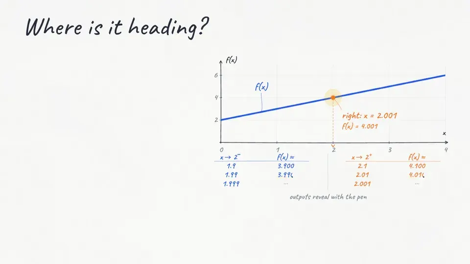
- Read a table from both ends toward and see which height both sides close in on. A table suggests a limit; it can never prove one, because it shows only finitely many inputs.
Transcript
1,037 words · 3 parts
Snapshots in a table
Sometimes you don’t get a graph at all, only a table of snapshots, like a camera’s frames, and this one is for a function h near x equals three. The trick with a table is to read it from both ends toward the middle. On the left, the inputs climb toward three, and h climbs from four point seven one through about four point nine seven and four point nine nine seven.
On the right, start at the far end, where x is three point one and h is five point three one. As the inputs move toward three, the outputs come down through about five point zero three and five point zero zero three.
Both sides are closing in on five, so we’d estimate that the limit is five. That nine in the middle is h of three, one snapshot at exactly three that the limit simply ignores. Notice I said estimate, because a table only shows you a handful of snapshots, and in a few minutes we’ll see exactly why that matters.
Here’s a calculator’s table for another function, k, near x equals negative one. Use it to estimate the limit of k of x as x approaches negative one.
Negative point nine nine nine sits on the right side of negative one, because it’s bigger. The plus sign on the negative one means inputs bigger than negative one, even when every one of them is a negative number.
Let’s build a table from our helicopter. At twenty-four frames a second the camera shows the blades creeping forward at twelve turns a minute, and we’ll call that the apparent spin. Call the frame rate F and the apparent spin S. As we dial up toward twenty-five, it slows to one point two, then to point one two, while the real rotor keeps turning three hundred times a minute, five every second.
Now come down from above twenty-five, and something strange happens. The blades creep backward, at minus twelve, then minus one point two, then minus point one two turns a minute, because each frame now comes a hair early, before a blade reaches its neighbor’s spot.
What do you think the apparent spin is heading for as the frame rate closes in on twenty-five from both sides? Right at twenty-five frames a second the apparent spin is exactly zero, and that’s the moment the rotor freezes.
When the snapshots lie
Why does it freeze? Here are six frames in a row, each one a twenty-fifth of a second after the last, and they’re identical. The rotor turns five times a second, so between two frames, a twenty-fifth of a second apart, it turns one fifth of a turn. With five blades, that drops every blade into the spot where its neighbor was a moment earlier.
Paint one blade tip yellow and you can catch it in the act. That yellow tip jumps a fifth of the way around in every single frame while the rotor seems to stand perfectly still. Every frame is accurate. What the frames miss is everything that happens between them, and a table of numbers can miss things in exactly the same way.
Here’s a table for cosine of pi over x, with snapshots at x equals plus or minus point one, point zero one and point zero zero one. Every single snapshot comes out to exactly one, from both sides of zero. Pi over point one is ten pi, five whole turns around the circle, so the cosine lands right back on one.
What do you think the limit of cosine of pi over x really is, as x approaches zero? Don’t take my word for it. Drag the probe anywhere between the table’s inputs, and let go to take your own snapshot.
Between the snapshots, the graph swings all the way down to negative one and back, faster and faster as x closes in on zero. No matter how far we zoom in, the swings never shrink, so the outputs never settle on one height. The limit of cosine of pi over x as x approaches zero does not exist.
Cosine of pi over x is a rotor that spins faster and faster as x gets close to zero. Our table was a camera that just happened to click only when the blade was back where it started.
Our calculator model takes snapshots too, one for every column of pixels across the screen, and then it simply joins them up. Zoom in on two, and the line runs straight through, even though the function isn’t defined there, because the hole falls between two columns of pixels. Now you fix it. Drag across the screen to slide the snapshots until one column lands right on x equals two.
Near zero, cosine of pi over x can swing several times between two neighboring columns. Each column catches a different part of that motion, so the screen draws a pattern that changes whenever we shift the window.
A graph on a screen is good evidence about a limit, but it’s never the final word. When something matters, look from both sides, check the function itself, and remember that a table is snapshots too.
Freeze it yourself
Let’s pull it together. Near any point, you read each side on its own, and the point on its own. The limit exists only when both sides head to the same height, and it never cares what’s sitting at the point itself. It fails to exist when the two sides disagree, when the outputs run off without bound, or when the function oscillates without ever settling. Graphs and tables are snapshots, so they let you estimate a limit, as long as you remember what can hide between them.
Now it’s your turn to freeze a helicopter. The camera’s running at twenty-two frames a second, so the blades are creeping forward. Turn the dial and close in on the frame rate that freezes the rotor completely.
One more. Make the blades creep backward at exactly one point two turns a minute. You can now explain exactly how a camera freezes a spinning rotor, and the next time a graph or a table tries that trick on you, you’ll know to look between the snapshots.