Topic 6.12: Integrating Using Linear Partial Fractions

Split the fraction

Let’s take a breather on a cliff you might remember from precalc. Every time you slide a new book in at the bottom, the tower leans a little farther out over the drop, but each new book buys you less reach than the one before. The fourth book bought an eighth of a book of reach, and the fifth bought only a tenth, so the drop between them is one eighth minus one tenth, which works out to one fortieth.

Combining fractions like that is the easy direction, and it works with letters too, because one over x minus one over x plus one combines into one over x times x plus one. We know how to combine fractions like these, so now let’s go the other way and recover the two simple pieces from the one fraction they make, and that trip backwards is called partial fractions.

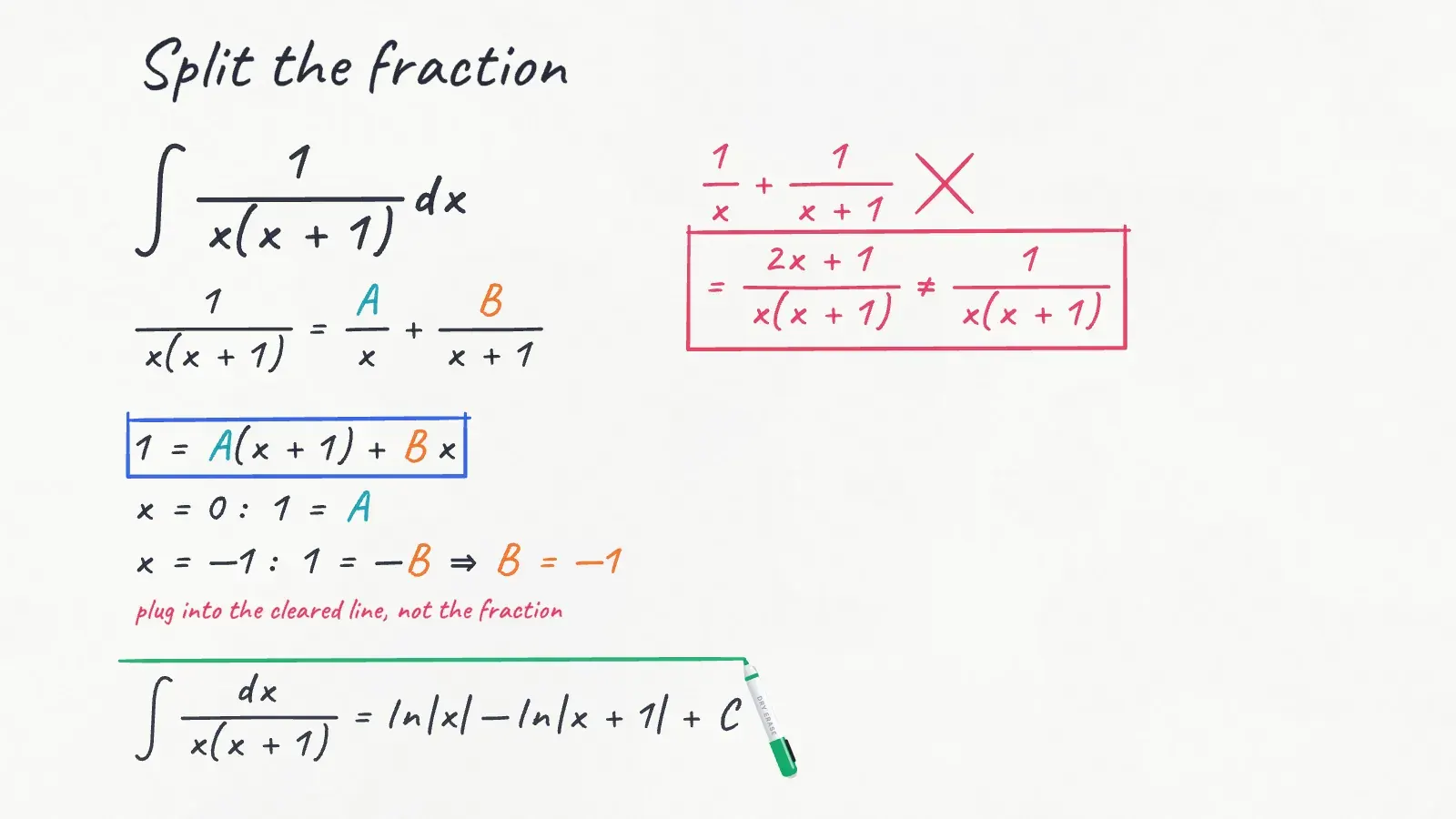
Now pretend you only had the right-hand side, one over x times x plus one. None of your rules can integrate it as it stands, but split into simple pieces, each piece is just a log. So let’s write it as A over x plus B over x plus one, and find A and B. Multiply both sides by x times x plus one to clear the fractions, and you get one equals A times x plus one, plus B times x.

That’s true for every x, so pick x’s that make terms vanish. At zero the B term disappears and A is one, and at negative one the A term disappears and B is negative one, the same split we combined a minute ago. Notice that we put zero and negative one into the cleared equation, never into the original fraction, where they’d mean dividing by zero.

The classic mistake is splitting it as one over x plus one over x plus one, but add those back up and you get two x plus one on top, so that’s a different fraction. With the right split, the integral is ln of the absolute value of x minus ln of the absolute value of x plus one, plus C. The absolute values are there because x and x plus one can be negative.

Out over the cliff, the target curve shoots straight up at the cliff edge, where x is zero. One piece is one over x, and the other, negative one over x plus one, hangs below the axis for every positive x. Together they land exactly on the target at every x except the two poles.

This curve is three x plus five over x plus one times x plus two. See if you can turn the A and B dials until your two pieces add up to it everywhere. Now you be the one who hides the pieces. Set A and B to any numbers you like and press combine, and the lesson will find them again from the fraction alone.

To get your pieces back, we clear the fractions. Plugging in negative one makes the B term vanish and hands back A, and plugging in negative two makes the A term vanish and hands back B, exactly the numbers that went in.

Factor first, then split

An exam question can hand you the bottom as a quadratic, so with x plus seven over x squared minus x minus six, the first job is to factor the bottom into x minus three times x plus two, and then we split and clear the fractions. Plugging in three gives ten equals five A, so A is two. Plugging in negative two gives five equals negative five B, so B is negative one.

That makes the integral two ln of the absolute value of x minus three, minus ln of the absolute value of x plus two, plus C. Now let’s put limits on our first fraction, from one to two, and a definite integral needs one check first. One over x times x plus one is continuous on that interval, because zero and negative one are both outside it, so the Fundamental Theorem of Calculus applies.

Evaluating ln x minus ln of x plus one from one to two gives ln two minus ln three, minus the quantity zero minus ln two. That simplifies to two ln two minus ln three, which is ln of four thirds, about point two nine.

Back on the cliff, between x equals one and x equals two, the piece above the axis is ln two and the piece below it is ln of three halves, so what’s left is ln of four thirds. Now try one yourself, the integral from zero to one of three over x plus one times x plus four.

Which tool?

On the exam nobody tells you which technique to use, so let’s sort these by their shape. For x times e to the x squared, I’d substitute for x squared, because its derivative supplies the x we need. For x times e to the x, I’d try parts, because differentiating x makes it disappear.

If the top is the derivative of the bottom, like two x plus one over x squared plus x, that’s substitution again. Swap that top for a plain one, and one over x squared plus x needs partial fractions. If the top’s degree is as big as the bottom’s, like x squared over x plus one, divide first. Which one of these needs partial fractions?

Fifty-two factorial, by hand

Now we can keep the promise, and for that we need the integral of ln x, which doesn’t even look like a product. The trick is to see an invisible one, so we write it as ln x times one, with u equals ln x and d v equals d x. Then d u is one over x d x and v is x, so u v minus the integral of v d u is x ln x minus the integral of one. That gives x ln x minus x, plus C.

Logs turn products into sums, so ln of fifty-two factorial is ln one plus ln two, all the way up to ln fifty-two, and since ln one is zero, that’s exactly the total area of these fifty-one bars. The bars hug the curve, so their area is close to the area under it, and the rectangle can measure that. On this picture the width is x and the height is ln x, so each horizontal strip on the left has area x times one over x d x, and adding those strips from one to fifty-two gives fifty-one.

The whole rectangle has area fifty-two times the natural log of fifty-two. Take away the fifty-one on the left, and about a hundred fifty-four point four six is left under the curve, exactly what our antiderivative predicted.

The bars poke up a little above the curve. How does ln of fifty-two factorial compare with one hundred fifty-four point four six? Each little sliver on top is almost a triangle, and if you slide them all together, they make about half the last bar, almost two more. That puts ln of fifty-two factorial at about a hundred fifty-six point four four.

If a number N is ten to the power p, then p is ln N divided by ln ten. Use your calculator to write fifty-two factorial as ten to some power, and tell me its first digit.

The real fifty-two factorial is about eight point oh seven times ten to the sixty-seventh, sixty-eight digits starting with an eight, so with one integral instead of fifty-one multiplications, you got the first digit right. Today you learned to trade an integral you can’t do for one you can. Parts runs the product rule backwards, partial fractions runs adding fractions backwards, and the shape of what you’re integrating tells you which one to grab. Both show up on the BC exam year after year, and the next time you shuffle a deck, you’ll know just how big the number in your hands really is.