Topic 6.3: Riemann Sums, Summation Notation, and Definite Integral Notation

No parachute

That speck is Luke Aikins, twenty-five thousand feet over California in the summer of 2016, and he has just stepped out of an airplane with no parachute and no wingsuit. Way down there, smaller than a postage stamp, is the one thing that can catch him, a net a hundred feet on a side. It hangs twenty stories up, between the tops of four cranes.

He falls for about two minutes, and near the end the air has settled him into a steady hundred and twenty miles an hour, more than fifty meters every second. A second or so above the net he rolls onto his back, and then he hits it. A little later, he climbed out of that net and walked away. Let’s replay the catch in slow motion and freeze it right in the middle.

At this instant the net is pushing up on him with about fourteen thousand newtons. But an instant has no time in it at all, and a push that lasts no time can’t slow anybody down.

Yet somehow all those instants together took a man falling at a hundred and twenty miles an hour and stopped him completely. A pile of nothings added up to something. By the end of this lesson, you’ll be able to take a whole curve of pushes like these and turn it into one exact number.

Then you’ll design the push yourself, we’ll drop him into your design, and we’ll see if it stops him. To get there, let’s hang a graph of that push in the sky, right next to the net.

Slice the catch

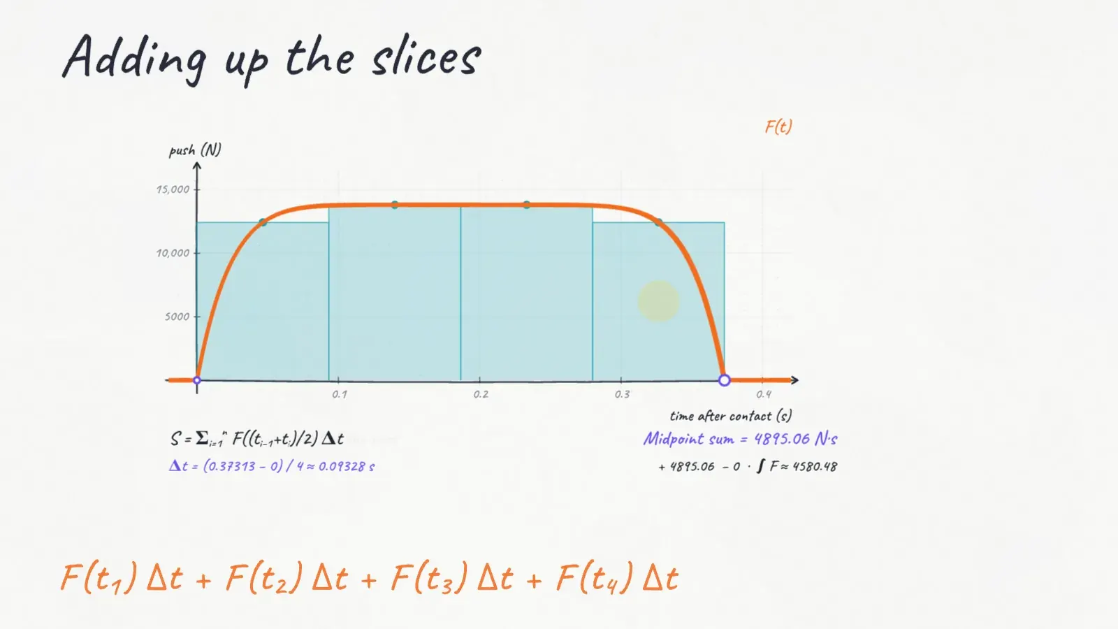
This curve is how hard the net pushes on him at every instant. It shoots up almost as soon as he touches the net, stays high while the net sinks under him, and drops back to zero as he stops. In our model, where we suppose the net sinks ten meters, the whole catch takes about thirty-seven hundredths of a second, and the push peaks near fourteen thousand newtons.

What matters for stopping him is how hard the net pushes and for how long. A steady push of ten thousand newtons for a tenth of a second counts as ten thousand times a tenth, a thousand newton-seconds.

If the push stayed steady we’d be done with one rectangle, but this push keeps changing, so no single rectangle can fit it. Let’s do the next best thing and chop the catch into four short slices of time. Inside each slice we’ll pretend the push holds steady at its value in the middle, a midpoint sum like the ones you built last time.

Each rectangle is one slice of the catch, and its area is a force in newtons times a sliver of time in seconds, one little push in newton-seconds. Add up the four little pushes and we get about forty-nine hundred newton-seconds, a decent estimate. But look at these corners sticking out past the curve, because they count push that never happened.

Make a guess first. As the slices get more numerous and thinner, does the total keep growing, shrink toward zero, or settle on one number? Then drag the slices up and find out, until you’re within ten newton-seconds of the true area.

Look at what happened. The corners shrank away, and the total stopped moving. Hold on to that number, and a little later we’ll find out why it had to come out to about that much.

Let’s write down what we just did, and there’s a much shorter way to say add up all these rectangles. With four slices, the total is the first push, plus the second, plus the third, plus the fourth, and each push is a force times the width of its slice.

Writing that out gets old fast, so we squash it into one big Greek letter, sigma, which is just a capital S, for sum. The little i is a counter that runs from one at the bottom up to four at the top. For each value of i, we take that slice’s force, F of t sub i, times its width, delta t, and add them all up.

With n slices instead of four, the counter just runs up to n. Each slice is T over n wide, where T, the length of the catch, is about point three seven three seconds. You met sums like this last time. They’re Riemann sums, and sigma is just a compact way to write one, a sum of products, each a height times a width.

Infinitely thin

Let’s watch a sum settle on a graph where we can check the answer, the line f of x equals two x, from zero to two. Four right-endpoint rectangles give a total of five, a little too much, because each rectangle’s corner pokes up above the rising line.

With eight rectangles the total drops to four and a half, and with sixteen it’s four and a quarter. Every time we double the slices, the extra area gets cut in half. Keep shrinking the slices and the totals close in on exactly four. That’s no surprise, because the region is a triangle with base two and height four, and half of two times four is four.

That settled number is what we were after. For a continuous function f on an interval, we define it as the limit of the Riemann sums as the number of slices goes to infinity. You saw this symbol last time. Leibniz invented it in 1675, and he took the S of sum and stretched it tall, because underneath it’s still a sum. Delta x becomes dx, a reminder that the widths keep shrinking.

We read it as the definite integral of f from a to b, where f of x is the integrand, and a and b are the limits of integration. That’s a second meaning of the word limit, and here it just means the place we start and the place we stop. For our line, the integral from zero to two of two x dx is exactly four, one number, not an estimate. Your slices can have different widths. Then the widest one has to shrink to zero too, or the sums can miss the integral.

Suppose we keep cutting the left part thinner and thinner, but that last slice stays a whole unit wide. Will the sums still close in on four?

Now let’s turn an integral back into a limit of sums. The exam loves this, so take the integral from two to five of x squared plus one, d x. We need the width of each slice first. The interval from two to five is three long, and cutting it into n equal slices makes each one three over n wide.

Now we need the sample points, at the right end of each slice, the exam’s usual choice. We start at two and take i steps of three over n, so slice i ends at two plus three i over n. Let’s check it. When i equals n we get two plus three, which is five, the right end of the whole interval. If we’d forgotten the starting two, we’d have landed on three.

Now we put that point into the function and multiply by the width. The integral is the limit of the sum of two plus three i over n, squared, plus one, all times three over n.

Now you go the other way. Use the one we just built as your guide, the width first, then the start, then the function, and pick the definite integral that equals this limit.