Topic 6.2: Approximating Areas with Riemann Sums

The wind won’t hold still

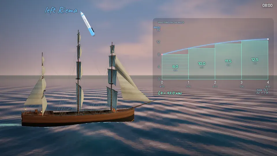
Real speeds don’t come in tidy steps, though. Out here the wind builds all night, so the ship speeds up minute by minute through the whole watch. The true speed traces out a curve. The navigator has four pegs, one for each hour, plus a fifth reading at eight bells. He holds each hour’s reading for the whole hour and adds up four rectangles.

When every rectangle takes its height from the left end of its interval, we call the sum a left Riemann sum. Riemann was born in eighteen twenty-six, about two hundred and fifty years after sailors started doing this.

Now look at the gold slivers above every rectangle. The ship kept speeding up after each reading, so every rectangle misses a little piece of the real area. Let’s see what that costs. This glowing ship is a ghost that sails exactly where the navigator’s sum says we are. By eight bells it’s fallen almost three nautical miles behind the real ship.

Take each height from the right end of its hour instead, and you get a right Riemann sum. Now every rectangle sticks up past the curve, and the ghost overshoots, more than two miles ahead of the ship. If you heave the log more often, each reading covers less time. The thinner rectangles hug the curve more closely, so the ghost closes in on the ship.

You take the log now. Using left or right sums, pick how often to heave it, so the ghost finishes within one nautical mile of the real ship at eight bells.

The navigator’s sum

Let’s do the navigator’s sum properly, the way the exam will ask you to. Here’s the log for the watch, the speed at the start of every hour, and at eight bells. Each interval is one hour wide. We call the left sum L four, for its four rectangles, and it takes the speed at the start of each hour times one hour.

That’s one times eight, plus one times ten, plus one times eleven and a half, plus one times twelve and a half, which comes to forty-two nautical miles. The exact area under the speed curve has its own name and symbol. We write it as the integral from zero to four of v of t, d t, and call it a definite integral.

The d t is there to remind you that every piece is a speed times a little bit of time. In the next lesson, we’ll define the integral exactly. Today we’re estimating it, so we write that it’s approximately forty-two. Now you find the right Riemann sum for the same watch, using the four one-hour intervals.

Which one is right? Neither of them, but we can say something better than that. The wind built through the whole watch, so v is increasing on the whole interval from zero to four.

When a function is increasing, every left rectangle uses the smallest speed in its hour, so it sits under the curve. Every right rectangle uses the largest, so it pokes above. The true distance has to be somewhere between forty-two and forty-seven. On the exam they’ll ask you to justify that, and a number alone won’t do it. Here’s how I’d write it.

Because v is increasing on the interval from zero to four, each left rectangle lies below the graph of v, so the left Riemann sum of forty-two underestimates the integral. There’s a tempting shortcut to watch out for. Left sums don’t always underestimate. If the speed were dropping, every left rectangle would stick out above the curve, and the left sum would be the overestimate.

For our navigator, the left sum is the dangerous one. It says forty-two miles when the ship has really come farther, so the coast is closer than he thinks. Which of these sentences would earn the justification point for saying the left sum is an underestimate?

Middles and trapezoids

Left and right trap the answer between them, but there are two smarter ways to use the log. On this watch the mate also heaved the log at every half-hour bell, so we know the speed in the middle of each hour too. A midpoint sum uses the speed at the middle of each interval as the height. Every rectangle cuts through the curve, a bit too high on one side and a bit too low on the other.

That’s nine point one plus ten point eight plus twelve point one plus twelve point eight, each times one hour, forty-four point eight nautical miles. A trapezoidal sum joins the readings at the two ends of each hour with a straight line, so each piece is a trapezoid. Its area is the width times the average of the two end speeds, so the first hour gives one times eight plus ten over two, which is nine.

Do the same for every hour and add them up, nine plus ten and three quarters plus twelve plus twelve and three quarters, forty-four and a half. Forty-four and a half sits right between forty-two and forty-seven. Each trapezoid averages a left height and a right height, so the trapezoidal sum is the average of the left and right sums.

Students mix these two up all the time. The midpoint sum plugs in the middle of the first hour, half an hour in, and reads the speed there, about nine point one. The trapezoid averages the two end speeds, eight and ten, to get nine. The midpoint reads the speed at the middle time, and the trapezoid averages two speeds, so they give different numbers.

Here’s a plain one with no ship in it. Use a midpoint sum with two equal subintervals to approximate the integral from zero to four of x squared, d x.

Which one comes out short? That depends on which way the curve bends, so let’s look at one that bends a lot. This curve bends downward, and we call that concave down. Here’s its trapezoid, with a straight top from one end to the other. How does this trapezoid compare with the true area under the curve?

The midpoint goes the other way. On a curve that bends down, the midpoint rectangle comes out a little long, because it covers more on the left than it misses on the right. Here the trapezoid gives thirteen and a half, the midpoint twenty and a quarter, and the true area is eighteen.

Our speed curve bends down too, just more gently. Put all four sums in order, and the true distance is squeezed between forty-four and a half and forty-four point eight. That’s a window less than a third of a mile wide.

When the rate goes negative

There’s one more thing the navigator has to think about before landfall. Across the harbor mouth there’s a sandbar, and the ship needs sixteen feet of water over it to cross, so he watches the tide. This graph shows how fast the depth over the bar is changing, in feet per hour, starting at six in the morning. At first the rate is positive, so the water’s rising, and after two hours it turns negative, so the water’s falling.

The area above the axis is a triangle, half of two times two, so the water rises two feet. The area below the axis is a triangle too, half of three times three, four and a half.

Because the rate is negative there, that’s four and a half feet of falling. Area below the axis counts as negative change, so over the five hours the depth changes by two minus four and a half, negative two and a half feet. The water over the bar was eighteen feet deep at six o’clock. How deep is it at eleven?

Joules from a curve

Speed isn’t the only rate that piles up into a total. This is a compound bow on a test rig, the kind archers hunt with. How much energy do you pour into it when you pull the string back?

As the string comes back, the gauge reads the force. It climbs to about two hundred newtons, and then the cams roll over and the pull gets easier, all the way down to about seventy at full draw. Force is a rate too, because it tells you how many joules each extra meter of draw adds. That makes the area under the force curve the total work, and newtons times meters gives joules.

Now try a left sum on this curve. While the force is rising the left rectangles fall short, but once it starts falling they stick out over the top. That means you can’t say ahead of time whether the whole sum is too big or too small. Rising or falling is what decides it, and this curve does both.

You run the test now, with six readings and no more. Put them where they’ll do the most good, and see if your trapezoids land within one joule of what the rig measured.

Real readings are rarely evenly spaced, so let’s do one on paper, the way it shows up on the exam. The first four gaps are a tenth of a meter, but the last one, from point four to point four eight one, is only point zero eight one meters. That means every trapezoid gets its own width.

The first trapezoid is a tenth of a meter wide, with forces of zero and a hundred thirty-four at its ends. Its area is point one times their average, six point seven joules. Finish it with the calculator. Use a trapezoidal sum with all five intervals to approximate the work done drawing the bow, in joules.

The six readings from the paper, both ends included, land within about two joules of the seventy-three point seven the rig measured. Now let’s spend them. Straight into the gold, fifty meters away.

Landfall

Back on the ship it’s seven bells, half past seven, and the sky ahead is starting to go gray. The navigator gets one last try before eight bells, and this time you choose everything.

This time you plan the navigator’s last try. Pick a kind of sum and how often to heave the log, using as few readings as you can, then commit and sail to eight bells. Land the ghost within a quarter of a nautical mile.

There’s the light on the headland, right where the sums said it would be, forty-four point seven nautical miles from where we started the watch. Look at what you can do now. When a graph shows a rate, the area under it is the total change, in the rate’s units times the input’s units.

When you can’t find that area exactly, you can estimate it with a left, right, midpoint or trapezoidal sum, and use the way the rate behaves to say when your estimate has to be too short or too long. On the exam, you’ll see a table of rates and the words, approximate using a trapezoidal sum. Now you know what every number in it means. You just did the navigator’s job, more than two hundred years later, and you’d have brought this ship home.