Topic 2.6: Competing Function Model Validation

The planet in the leftovers

It’s late on the night of September the twenty-third, 1846, in the dome of the Berlin Observatory, and two astronomers are about to point this telescope at a patch of sky where nobody has ever noticed a planet. They’re doing it because of a letter from a man in Paris they’ve never met. And his reason for writing starts with this brass machine. It’s a model of where every planet should be, on any night you like.

This glass bead is where Uranus really was in the sky, year after year, and the brass one is where the model said it would be, and for forty years the two of them stayed together. Then, a few years after 1821, the real planet started slipping behind, a little more every year and always the same way, by an amount so tiny that we’ve had to magnify the gap many times over just to see it.

Some astronomers wondered whether gravity itself worked differently that far out, but a young French mathematician named Urbain Le Verrier decided the leftovers were a message, that something nobody had ever seen was pulling Uranus back, and he worked out where. That’s what his letter says.

By the end of this lesson, you’ll be able to read what any model leaves behind. You’ll tell whether it’s missing something. And you’ll tell which way it’s wrong. At the very end, you’ll use that to find the planet yourself.

What a model leaves behind

His model was built on Newton’s gravity, but the move he made works on any model at all, so let’s stop the clock in 1840 and look closely. The model says Uranus should be right here at the brass ball, but the sky says it’s actually back here at the glass one, and the gap between them is what the model left behind.

That leftover is called a residual, and you always find it the same way, by taking the actual value and subtracting the value the model predicted. Uranus moves forward along its orbit, this way, so the angle that gives its position keeps growing. The real planet is behind the brass one, so I’d like you to work out what that means for the residual.

So in 1840, what’s the sign of the residual? And what was the model doing? Now let’s ride along with the model, so the camera follows the brass Uranus and it never moves on screen. Everything the model got right disappears and only the leftover still moves, and soon we’ll do the same thing to a graph.

So here’s the definition. A residual is the actual value minus the value the model predicted, and the order matters, because it’s what makes the sign mean something. If the residual is positive, the real value came out above the prediction, so the model was too low and underestimated. If it’s negative, the model was too high and overestimated, exactly what happened with Uranus. The most common slip is doing the subtraction backwards, so every time you write a residual, say it in your head, actual minus predicted.

Three experts, one table

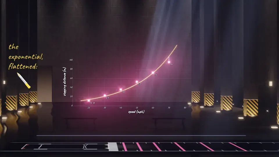
Now let’s give the models you’ve been building all unit a real job. Every learner driver in Britain memorizes this table, how far a car goes before it stops at each speed. The distance grows by eleven meters, then thirteen, then seventeen, twenty and twenty-three, so the rate is changing, but only slightly, and when it changes that gently, a line, a parabola and an exponential can all fit the data.

So let’s hire three experts. The first fits a line, the second a parabola, the third an exponential, which is what your calculator does with LinReg, QuadReg and ExpReg, and look, all three of them hug these six points.

But ask them about something the table doesn’t cover, like stopping from a hundred miles an hour, and they stop agreeing. The line says a hundred forty-one meters, the parabola a hundred eighty-four, and the exponential three hundred sixty-nine. All three came with impressive correlations, so those numbers can’t settle it. We’ll do what Le Verrier did instead, and look at what each model leaves behind.

Subtract the model

Let’s take the line on its own. Every point hangs from it by a thread running straight up or down, and each thread is a residual. At this scale they’re tiny, and at seventy miles an hour the real stop is five meters longer than the line said, a gap you can barely see.

Now let’s ride along with the line, the way we rode the orrery. Watch it lie down flat, and every point ride down with it, keeping exactly its own thread. Then we stretch the picture up and down by eight so the leftovers are big enough to read, and there’s a smile, high at both ends and low in the middle. That smile is the curve the line failed to follow.

This picture is called a residual plot. The inputs run along the bottom, and the residuals go up the side. In other words, it’s still the same data. Nothing is thrown away. We’re just looking at it from the model’s point of view.

To decide whether a residual plot has a pattern, ask whether you could guess where the next point would land. Here you can, it would be up high at eighty, and that means the model missed something. So the line is out, even with a correlation of point nine nine one. The exponential is next. Before I lay it down, I want your guess.

I’ll flatten the exponential and stretch it by eight. What shape do you think its leftovers will make? Now the parabola, the same flatten, and because its leftovers are so tiny, a much bigger stretch, forty times this time, and look what’s left. Almost nothing is left. A few scraps, less than half a meter, scattered with no shape at all, and if I asked you where the next one goes, you’d have no idea.

That’s what the right model looks like. When the residual plot appears without a pattern, the model has caught the shape of the data and only noise is left, so we say the model is appropriate. Smile, nothing, frown. A parabola is really a line with a bend in it, so let’s go back to the straight line and give you the bend.

Grab the line and bend it, slowly, and keep going until the leftovers stop making a shape. Too little bend leaves a smile, too much leaves a frown, and right in between, the pattern disappears.

The leftovers picked the parabola, and a good model should make sense in its context too, so let’s check. A parked car needs no road at all to stop, so a sensible model should give about zero at zero miles an hour. The line says negative twenty-six point six meters, the exponential says a parked car needs six point three meters to stop, and the parabola says about half a meter, which is about as close to zero as the table’s rounding allows.

And there’s a reason it’s a parabola. You might remember from the night road in lesson 1.3 that thinking distance grows with speed but braking distance grows with speed squared, so the total is a parabola. In fact, run the same regression in feet and you get a parabola that matches v plus v squared over twenty to within about a foot at every speed, and that’s the rule the Highway Code uses to make the table in the first place.

Which way would you rather be wrong?

Even the best model is a little wrong, so it’s worth asking which way it’s wrong. Sometimes we care about the signed residual, which says whether the model ran high or low, and sometimes only about its size, how far off it was. Compare the line to the parabola, our best model, and you’ll see it isn’t wrong the same way everywhere. It underestimates below about twenty-eight miles an hour, overestimates in the middle, and underestimates again above about sixty-two.

That last stretch is the dangerous one. A driver who trusts the line at a hundred miles an hour expects to stop in a hundred forty-one meters and actually needs a hundred eighty-four, so they slide forty-three meters past the line. So for stopping distances, you’d much rather have a model that overestimates. The error that costs you is the one that comes up short.

Weather forecasters lean the same way. A study found that when The Weather Channel said twenty percent chance of rain, it rained only about five percent of the time. That’s a bias forecasters defend, because people forgive an umbrella they didn’t need far more easily than a soaking. Your phone predicts how many hours of battery you have left. If it has to be wrong, which way would you rather it was wrong?

A young country, no hints

Here’s a table with no hints at all about what kind of model it wants. It’s the population of the United States in every census, from 1790 to 1860. First the differences, each count minus the one before. They grow faster and faster, from one point three eight up to eight point two five, so a line is in trouble. Now the ratios, each count divided by the one before. They barely move, about one point three four every ten years, which smells like an exponential.

A smell isn’t proof, so let’s run all three regressions and let the leftovers decide. Look at the line first. Its leftovers make a smile again, just like the stopping distances did. The parabola does much better, but its leftovers still rise and fall in a wave. Notice the scale shrank, because these leftovers are all under a million.

And the exponential’s leftovers are smaller still, a quarter of a million at most. They leave nothing you could predict. And the context agrees, because a young country with lots of children and immigrants grows by about the same percentage every year, about three percent, and growing by a constant percentage is exactly what exponentials do.

Now let’s use it. Ten years past the end of the table, in 1870, the model predicts about forty-two million people, and the census counted thirty-eight point six million. What’s the model’s residual for 1870, in millions?

And like Uranus, that residual is carrying a message. Between 1861 and 1865 the country fought the Civil War, with hundreds of thousands of deaths and fewer births and immigrants, and the war is sitting right there in that gap.

Is it really exponential?

One more table, and this one’s yours, the total number of Pokémon after each new generation of games, from a hundred fifty-one in 1996 to one thousand twenty-five in the generation that began in 2022. There are more and more every game, so it feels like it’s exploding, and plenty of people would call it exponential. Here are both models with their leftovers.

Take a good look at both residual plots. Then you decide. Which model is more appropriate for the Pokédex? And what’s the reason? And the context agrees, because a design team adds roughly the same number each game, about a hundred, or about thirty-three a year.

This is exactly how the AP exam asks it, and it wants the reason in words, like the linear model is appropriate because its residual plot appears without a pattern. On the 2025 exam, a reason like “the r value is high” earned nothing, so the reason has to come from the data itself, like its residual plot or its ratios.

The exam has also asked why a model’s error grows, and on the 2024 exam fewer than one student in ten could explain it. The answer that earns the point says how the model and the data pull apart, like a sales model that keeps climbing after the real sales start to fall, so the leftovers keep growing, just as Uranus’s did after 1821.

Back to 1846

So let’s go back to 1846 and the leftovers that started it all. Le Verrier did exactly what you did with the bend. He added the missing piece to the model, and here the missing piece is a planet.

He had to work out where that planet was from Uranus’s leftovers alone. We’ve fixed how far out it is and how heavy it is, so all you need is where it was in 1846. Drag the new planet around the orrery until the strip of leftovers goes completely flat.

Le Verrier sent that position to Berlin, and on the night his letter arrived, Johann Galle and a student named Heinrich d’Arrest turned this telescope to it. At the eyepiece, Johann Galle read out the stars he could see, one at a time. The student checked each one against a brand-new star chart of that part of the sky. And in less than an hour, the student shouted, “That star is not on the map!” It was Neptune, less than a degree from where Le Verrier said it would be.

Two days later Galle wrote to him, “The planet whose position you predicted really exists.” A man had found a planet by reading the leftovers of a model, without looking through a telescope himself. To be fair, he got the planet’s distance wrong and was a little lucky that it sat where he said. And when he tried the same trick on Mercury, the planet he predicted never turned up, because the missing piece there was Einstein’s relativity.

What to remember

So, to recap, a residual is the actual value minus the predicted one, and its sign tells you which way the model missed, positive for an underestimate and negative for an overestimate. To check a model, subtract it, then look at the residual plot. If you can’t predict where the next point will go, the model has caught the shape.

Then ask the context, whether the data adds the same amount or multiplies by the same factor, and which mistake would hurt more. That’s how Le Verrier found a planet. And now you can read the leftovers the same way.