Topic 1.13: Function Model Selection and Assumption Articulation

The race that ends before the gun

What you’re looking at is every Olympic men’s hundred-meter champion since eighteen ninety-six, lined up for one race, and each of them is about to run it in exactly the time that won them gold. And they’re off. Each one is matched to his real gold-medal time, from twelve seconds in eighteen ninety-six down to Bolt’s nine point six three.

Bolt wins, of course, and the eighteen ninety-six champion is still more than twenty meters back, with a whole century of sprinting strung out between them. In two thousand four, four scientists published a short paper in the journal Nature, and they drew a straight line through a century of these winning times, one for the men and one for the women.

The women’s times had been dropping faster than the men’s, so their line is steeper, and if you follow both lines into the future, sooner or later they cross. By their math, at the Olympics of twenty-one fifty-six, the women’s champion runs it in just over eight seconds and beats the men’s champion for the first time in history.

Then a statistician named Kenneth Rice wrote back with an even better race, because if you keep following the same line, somewhere around twenty-six thirty-six the winning time drops below zero. So let’s watch the race of twenty-seven hundred.

Look at the clock. The winner crossed the finish line a full second before the gun went off. By the end of this lesson, you’ll be able to look at data like this. You’ll choose the right kind of function for it. And you’ll say exactly where it stops telling the truth.

That last part matters more than you’d think, because on the twenty twenty-five AP exam it was worth a point that almost nobody in the country earned. A straight line wasn’t a crazy choice for their data. So where did it go wrong? First we need a way to tell what kind of function made a list of numbers.

Three lists of numbers

Here are three lists of numbers, and each one counts something real. I’m not telling you what yet. I want you to work out what kind of function made each one. In the first list, the input goes up by one each time. So let’s look at how much the output changes on each step.

Two minus one is one, three minus two is one, and it’s one every single time. The same change for every equal step means a constant rate of change, and that’s exactly what a linear function has.

The second list changes by one, two, three, four and five, so it isn’t linear, but the changes themselves go up by exactly one every time. Take the differences again and you get one, one, one, one, and just like the cannonball in lesson one point three, constant second differences mean a quadratic.

The third list is sneakier. Its first differences are one, two, four, seven and eleven, its second differences are one, two, three and four, and only on the third round do we finally get one, one, one.

So this one is a cubic. It’s the rule you met in lesson one point five. With equal steps in the input, the first column of differences that holds still gives you the degree. Measured data, like race times, are never this tidy, so we look for differences that are roughly constant, and that word, roughly, matters a lot today.

Picking the type is only half of an AP question. On the twenty twenty-five exam, students also had to give a reason based on how the outputs change as the inputs change, and most of them lost that point. Saying that the graph looks curved, or that a regression fits, earns nothing, because lots of graphs curve, and a calculator will fit a quadratic to anything you give it.

This table’s inputs go up by one and its outputs are three, five, eleven, twenty-one, and thirty-five, and it’s a quadratic. Which reason would earn you the point?

Bread, pizza, cake

So what were those lists counting? Let’s find out somewhere cozier than a stadium, a little pizzeria at eleven at night, with the wood-fired oven still going. The first list was a breadstick, where every cut adds exactly one more piece, so n cuts give you n plus one pieces, a constant rate of one piece per cut.

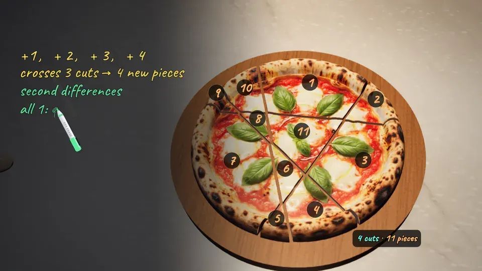
The second list was a pizza with straight cuts. You want as many pieces as you can get. One cut makes two, and a second cut across it makes four. Three straight cuts can make seven pieces of this pizza, not just six, so try dragging the cuts around until you find all seven.

A fourth cut that crosses all three makes eleven pieces, which surprises almost everybody, because cutting through the middle the normal way only gets you eight. The list grows this way because each new cut can cross every cut already there, so the first cut adds one piece, the second adds two, the third three and the fourth four.

It’s the same reason three cuts made seven, because a fourth cut that crosses three others gets chopped into four segments, and each segment splits one piece in two. The rate goes up by the same amount every time. And that’s exactly what makes a quadratic. The third list was a birthday cake, cut with flat cuts at any angle. Three cuts give you eight pieces.

Four cuts give you fifteen. That’s a lot of cake for four cuts. The cake grows for the same reason, because every new flat cut gets sliced up by the cuts already there, just like a pizza, so the third cut adds four pieces and the fourth adds seven, and one, two, four, seven is the pizza list itself.

Look at what we found. A breadstick is basically one-dimensional and its list is linear, a flat pizza has two dimensions and its list is quadratic, and a cake has three and its list is cubic. Areas grow in two dimensions and volumes in three, and that settles the most important question in any pizzeria.

Here are two twelve-inch pizzas and one eighteen-inch pizza. Which gives you more pizza? So the context can tell you the type. So can the differences, and the best answers use both.

Dimensions, points and turns

Here’s the version to remember for the exam. A problem about area, anything two-dimensional, often calls for a quadratic, and a problem about volume, anything three-dimensional, often calls for a cubic. In fifteen ninety-one, the mathematician Thomas Harriot worked out how many cannonballs fit in piles like this one. Piles with one to five layers hold one, five, fourteen, thirty, and fifty-five balls, so what degree of polynomial models the pile?

The differences also hold a warning. Through any two points with different inputs there’s always a line, and through any three there’s always a parabola, or a line if they happen to line up.

So what about six points? Take the six women’s times the paper used, from nineteen eighty-four to two thousand four, and difference them five times, and the fifth column has only one number left, and one number is always constant.

It’s the same rule as before, because a column that holds still is exactly what a polynomial makes. Still in the first differences means a line, in the second a parabola, in the third a cubic, and still in the fifth means degree five. You can run that table back up from the one number and rebuild all six times, so some polynomial of degree five or less passes through any six points with different inputs, perfectly.

So a perfect fit, on its own, tells you nothing. It doesn’t say whether the model is any good. Hold on to this curve. We’ll take it back to the stadium. And we’ll see what it predicts.

The shape of the data helps too. A halfpipe has one lowest point and it’s symmetric, and data like that, roughly symmetric with one maximum or minimum, call for a quadratic. A double bowl, with two low points and a hump between them, turns three times, but a quadratic only turns once and a cubic at most twice, so it needs a polynomial of at least degree four. In general, several zeros or several peaks and valleys point you toward a higher-degree polynomial.

One rule, then another

Back to the stadium, because one race deserves a closer look, Usain Bolt’s world record in Berlin in two thousand nine, nine point five eight seconds. Watch his distance against the time. For the first few seconds he’s still speeding up, so each ten meters takes less time than the last, and the graph bends.

But by about fifty meters he’s running at nearly top speed, and from there to the finish every ten meters takes him about point eight two seconds. It isn’t exactly the same every time, but it’s roughly the same, so that part of the graph is roughly a straight line, about twelve meters every second.

So one race has two different behaviors on two stretches of time, and that’s what a piecewise-defined function is for, different functions on intervals that don’t overlap, used whenever the rule changes partway through. You’ve seen one before, in lesson one point two, where the Falcon nine’s fuel drained at one rate, then a slower one, then the first again, three lines glued together.

Your phone goes from zero to fifty percent in twenty-six minutes, from fifty to eighty in the next thirty-one, and from eighty to a hundred in eighty-three more. What kind of model fits that best?

Say the bet out loud

Now back to that paper. Every model is a bet on what stays the same, and those scientists made one when they drew their line. Their line bets that the winning time drops by the same amount every year, about seventeen thousandths of a second, which is a bet about how the year and the time change together. And to be fair, they said so. Their paper says the lines cross in twenty-one fifty-six if current trends continue, and that little if is the whole assumption.

An assumption can even decide the type of function. Say a chocolate company makes its bunny twice as tall, and you want to know how much more chocolate it needs. If the bunny is solid, the chocolate is a volume, so it takes two cubed, eight times as much. But most are hollow, and if the shell stays just as thick, the chocolate is really an area, two squared, only four times.

Same bunny, same question, and one assumption turns a cubic into a quadratic. So when the AP exam asks for a model’s assumptions, say what the model bets stays the same. A restriction is different, it’s where the bet is allowed to be used.

Where the bet runs out

Let’s test the perfect fit from a few minutes ago. The degree-five curve through those six times from nineteen eighty-four to two thousand four. So what does this perfect curve predict for the Olympics of two thousand eight?

Thirteen point one seconds. The real champion in two thousand eight ran ten point seven eight, and the perfect curve’s champion comes jogging in more than two seconds later. By two thousand twenty-four it predicts a hundred thirteen seconds, which is a nice stroll. Inside its data the curve is perfect, and outside its data it’s nonsense. The honest way to use a model is to trust it only where you have data, so the floodlights should only light the years where somebody really raced.

Drag the edges of the floodlights. Make them light only the years where this line can be trusted. Outputs can be impossible too. A winning time can’t be zero or negative, so the line’s outputs have to stop before twenty-six thirty-six even if you ignore the domain.

That’s a range restriction, and they’re everywhere. A battery can’t pass a hundred percent, people come in whole numbers, and sometimes the context even tells you which way to round. A national test once asked how many buses it takes to carry eleven hundred twenty-eight soldiers, thirty-six to a bus. Most students divided correctly, but only about a quarter answered thirty-two, the smallest number of buses that gets everyone on board.

The point almost nobody got

Now for the AP question I promised you. On the twenty twenty-five exam, a question gave the total number of times a song had been played, in thousands, and modeled it with a quadratic. The model rises, reaches its maximum at t equals eleven months, and then turns around and starts going down. Part c asked something new. How could that maximum set a boundary for the model’s domain, based on the context?

Think about what this counts. It’s the total number of plays, every play since the song came out, so can a total like that ever go down? It can’t, because nobody can un-play a song. So once the model starts decreasing after t equals eleven, it’s describing something impossible, and t equals eleven is the right edge of the domain.

For full credit, you’d write that the total number of plays can never decrease, but the model decreases after its maximum at t equals eleven, so the domain should end at t equals eleven. Only about one student in twenty earned that point, and now you could write it in your sleep.

Call it before it breaks

So let’s go back to the race that ended before the gun. Let’s describe it properly. A line was a fair choice, because the times were dropping at a roughly constant rate. It assumes the same drop every year, its domain is nineteen twenty-eight to two thousand four, where the data are, and its outputs must stay above zero, because a race takes time.

Which means the race of twenty-seven hundred never gets run. And this is what really happened next. Every women’s champion since the paper has run slower than its line, and the times are leveling off, which a straight line can never do. The statistician George Box said it best, all models are wrong, but some are useful, and now you can pick a useful one and know exactly where it stops being useful.