
Topic 1.4 key terms
- polynomial function
- A function equivalent to , where is a whole number () and each is a real number: every term is a number times to a whole-number power. Constant functions count too. Factored forms count.
- degree
- The highest power of x in a polynomial ( in the general form). The landing has degree 3.
- leading term / leading coefficient
- The term with the highest power, , and its coefficient . From a factored form, multiply the leading piece of each factor: .
- rate of change (of a landing)
- How many metres the height changes per metre along the ground: the tilt of the snow. Negative while the landing falls, zero where it is level, positive where it rises.
- local (relative) maximum / minimum
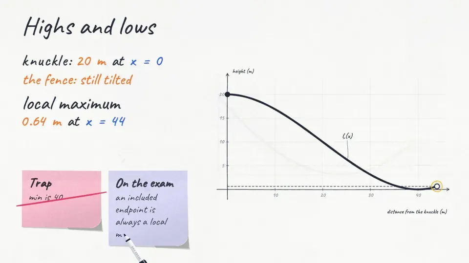
- An output value where the function switches from increasing to decreasing (max) or from decreasing to increasing (min), or at an included endpoint of a restricted domain. The max or min is the OUTPUT (a height); say where it occurs separately.
- included endpoint
- An endpoint that belongs to a restricted domain, such as x = 44 in 0 ≤ x ≤ 44. It is a local maximum or minimum even when the graph is not level there (the fence).
- global (absolute) maximum / minimum
- The greatest output of the function on its whole domain (global maximum) or the least output (global minimum). It can occur at more than one x. On 0 ≤ x ≤ 44 the landing's global max is 20 m at x = 0 and its global min is 0 m at x = 40.
- concave up / concave down
- Concave down: the rate of change is decreasing (the graph bends down). Concave up: the rate of change is increasing (the graph bends up).
- point of inflection
- An input where the rate of change switches from increasing to decreasing or from decreasing to increasing, so the graph switches concavity. On a landing that falls from concave down to concave up, it is the steepest point: the sweet spot.
Transcript
2,523 words · 8 parts
The sweet spot
This is a big-air jump, a ramp of steel and snow as tall as a twenty-story building, built in the middle of an old steel mill. A rider drops in, hits the kicker at more than eighty kilometers an hour, and for a couple of seconds she’s flying. Right now she’s thinking about one thing, where she’s going to land, and there are three very different places she could come down.
Riders have a name for one of these spots, the sweet spot. Land there and it feels like stepping off a curb, but land on either of the other two and it’s more like stepping off a roof. So which one do you think it is?
And she lands right on the steepest part, as soft as anything. Now watch the same jump again, but this time she comes up short and lands on the knuckle, the rounded edge at the top. And this time she flies too far and lands in the flats.
On the steep part the snow falls away under her almost as fast as she falls, so she slides into it. On flat snow the whole fall stops at once, like stepping off the roof of an eight-story building. By the end of this lesson, you’ll take the equation of a jump like this one and find the one spot a rider wants to land. You’ll find the two spots that hurt, too. And you’ll do it before anyone drops in.
And that’s not a figure of speech. The official rulebook for ski jumps builds the top of a landing hill out of a polynomial. So let’s start where the builders start, with the shape of the snow.
The snow has an equation
From the side, the landing is a curve, so let’s put axes on it. x runs along the ground from the top of the knuckle. The height is measured above the flats, and both are in meters.
The rulebook says the top of a ski-jump landing should be a cubic curve, and this one is too. Its equation is L of x equals one over sixteen hundred, times x minus forty squared, times x plus twenty.
Let’s take that equation over to the board. So, what’s inside it? This is called factored form, and it hides how the polynomial is built, so let’s multiply it out. First, x minus forty, squared, is x squared minus eighty x plus sixteen hundred.
Times x plus twenty, that’s x cubed, plus twenty x squared minus eighty x squared, minus sixteen hundred x plus sixteen hundred x, plus thirty-two thousand. The two x terms cancel, and twenty x squared minus eighty x squared is negative sixty x squared. And dividing by sixteen hundred gives one over sixteen hundred x cubed, minus three eightieths x squared, plus twenty.
That’s a polynomial, because every term is a number times x to a whole-number power, all added together. The biggest power is three, so L has degree three, one over sixteen hundred x cubed is its leading term, and the number in front, one over sixteen hundred, is its leading coefficient.
And you didn’t have to multiply anything out, because the leading term is just the leading pieces multiplied together, one over sixteen hundred, times x times x, from x minus forty squared, times one more x. Not everything with an x in it is a polynomial, though. Two to the x, one over x, and the square root of x don’t count. None of them is x raised to a whole-number power.
Now you try one. What’s the leading coefficient of g of x equals x squared, times four minus x, times two x plus one?
Tilt is the rate
Now let’s go back out on the snow. The equation hides the thing a rider cares about most, which is how steep the landing is at every point. This sled carries a ruler that lies flat against the snow. So the ruler’s tilt is the snow’s tilt, and the number on its readout is the rate of change of the height, how many meters the height changes for each meter you go forward.
On top of the knuckle the ruler is level, so the rate is zero. As it slides over the edge, the snow tips down and keeps getting steeper, a quarter of a meter down for every meter across, then half a meter, then more than six tenths.
So where does it stop getting steeper? Grab the sled, drag it to the steepest snow you can find, and keep an eye on that rate.
Past that point the snow gets gentler and gentler, until down in the flats it’s level again and the rate is back to zero. Then it tips up toward the fence, so the rate turns positive, about a third of a meter up for every meter across.
So the landing falls from the knuckle all the way to the flats. It only rises on the last little stretch. The two level places, the knuckle and the flats, are the two spots that hurt. Now let’s put the whole landing on the board. We’ll give everything we just saw its name.
Highs, lows, and the fence
Here’s the same landing as a graph. x goes along the ground, and the height goes up. In function words, L is decreasing from zero to forty and increasing from forty to forty-four. At forty the graph switches from decreasing to increasing, so the snow there is lower than everything around it, which makes it a local minimum.
On the exam you’d say L has a local minimum of zero meters at x equals forty, with the height first and the place second. The minimum is the height, zero meters, and forty is where it happens. Writing “the minimum is forty” loses the point, because forty is a place on the ground, not a height.
Look up at the knuckle. L is twenty meters at x equals zero. That’s the highest snow on the landing. Now look at the fence at the far end. The snow there is still tilted, so you’d think it can’t be a maximum.
But the landing stops at forty-four, and nothing near the fence is higher than it, since everything just to its left is lower. So the fence is a local maximum, zero point six four meters at x equals forty-four.
An included endpoint of a restricted domain is always a local max or min, even when the graph isn’t level there, and the exam loves restricted domains. Out of all the snow, the knuckle’s twenty meters is the highest, so that’s the global maximum, and the flats’ zero is the lowest, the global minimum. Now look at the whole landing. Which of these statements is true?
But the equation doesn’t know where the snow stops, so if x can be any real number, the graph keeps going, down forever on the left and up forever on the right, and the knuckle becomes a real turn. So over all real numbers L has no global maximum or minimum at all, and that has to do with its degree being odd.
Where the rate turns around
Now the rate gets its own graph. A point will slide down the hill. Right underneath it, we’ll plot its rate of change. One value for every x. It starts at zero on the knuckle.
Then it dives as the snow gets steeper, and bottoms out. It climbs back to zero in the flats, and goes positive on the way up to the fence. And look where it bottoms out. The rate is lowest at x equals twenty, exactly where the snow is steepest.
Before twenty, the rate is decreasing, so the snow keeps getting steeper and the hill bends down like a dome, concave down. After twenty, the rate is increasing, the snow gets gentler and the hill bends up like a bowl, concave up. The place where the bend switches is called a point of inflection, and on a landing, that’s the sweet spot.
A point of inflection is where the rate of change switches between increasing and decreasing, which is the same as the graph switching between concave down and concave up. And look at the stretch from twenty to forty, where the hill is still going down but getting gentler. It’s decreasing and concave up at once, a combination a lot of people get wrong, and it starts right at the sweet spot, where riders land.
Or picture a little car driving along the curve. Over the knuckle you’re steering right, then you straighten out bit by bit until at x equals twenty the wheel is perfectly straight for an instant, and then you steer left. And notice that twenty is exactly halfway between the knuckle and the flats. That happens on every cubic that turns twice, but don’t count on it for anything else.
There’s one more trap here, and it catches a lot of people. Here’s a slope with a level ledge halfway down. It’s level, just like the knuckle and the flats, so what kind of point is it?
It’s neither, because the snow is going down before the ledge and still going down after it. The rate touches zero but never switches sign, so for a point inside the domain, a level spot isn’t enough, and the rate has to switch sign.
On the exam, you’ll often get a table instead of a picture. So here are the landing’s heights every eight meters. From twenty at the knuckle down to zero in the flats. From zero to eight, the height drops from twenty to seventeen point nine two, about two meters over eight, so the average rate is negative zero point two six. From eight to sixteen it drops almost five meters, so the rate is negative zero point six two, steeper.
Then it drops almost six meters, negative zero point seven four, then about five, negative zero point six two, and about two, negative zero point two six. So the rates fall and then rise, and the steepest stretch is from sixteen to twenty-four, so that’s where the bend switches and the point of inflection has to be. This is exactly how the exam asks it. Here’s a table for a different cubic, g. Where does the graph of g change from concave down to concave up?
The valley in the fog
Now let’s go somewhere completely different, a high valley at sunrise, with fog lying in the low ground. Say you drop a marble here. It only knows which way is downhill right where it’s sitting, so it rolls that way, and stops in the first hollow it finds, where downhill switches to uphill, a local minimum.
That’s the simplest picture of how a lot of artificial intelligence learns. It feels which way is downhill on a landscape of its own mistakes, takes a small step, and does it again hundreds of thousands of times, and it can run into exactly this marble’s problem. Look at this marble, stuck in its hollow. It can’t know whether there’s a deeper one somewhere else in the fog.
So now the marbles are yours. Drop as many as you like, wherever you like, and find the lowest point in the whole valley.
Now look at the water line, because it’s the zero line of this valley’s polynomial, so every shore is a zero. Every lake lies between two shores, and between two shores the bed has to dip to a deepest point, even when you can’t see it. Michel Rolle proved back in 1691 that a polynomial has to turn around between any two of its zeros.
Now let’s raise the water until the hill goes under. The two lakes become one, and between its two shores the bed dips down twice, so the rule only promises at least one turn. And if we drain it instead, the small lake disappears but its hollow is still there, a turn with no shores at all, so the rule only works one way. Two shores always mean a turn, but a turn doesn’t need shores.
And there’s one more thing you can only see from far away. Both ends of this valley climb into mountains and keep climbing, so somewhere in between there has to be a lowest point of all. On every polynomial of even degree, the two ends go the same way. This one has degree four and a positive leading coefficient, so both ends go up and it has a global minimum.
Now turn the whole valley upside down. Its leading coefficient is negative now, so both ends plunge, and there’s a global maximum and no global minimum at all. Now flip it back. Both ends climb again.
A cubic, like our landing’s, is different. It has odd degree, so one end falls forever and the other climbs forever, and that’s why it has no global max or min at all. So here are the two rules in exam language. Between any two distinct real zeros of a polynomial, there’s at least one local maximum or minimum.
And a polynomial of even degree always has either a global maximum or a global minimum, which for a quadratic is right at the vertex. Both show up on the exam as must-be-true questions.
A jump nobody’s ridden
Let’s go back to the steel mill. The builders have just finished a brand-new landing that nobody has ridden yet. Its equation is up on the big screen. This one’s a quartic, so it bends a little differently than the first landing did.
So before anyone drops in, find the sweet spot. The screen has this landing’s survey, every four meters, so drag the flag to the spot where a rider wants to land.
So let’s send someone down the new landing. And she lands right on the flag, as soft as the first one. Now two more riders. One comes up short, on the knuckle at the top. The other flies too far, into the flats at the bottom. Both spots are level, and both of them hurt.
And because this equation has even degree and a negative leading coefficient, both ends go down, so it has to have a global maximum. It’s the knuckle’s fifteen meters, higher than anywhere else on the whole curve. You just did what the people who build these jumps do. From one equation you found the spot a rider wants to land and the two spots that hurt, before anyone dropped in.
What the snow told us
Here’s the first landing one last time. Its degree and leading coefficient come straight off the equation, even in factored form. A max or min sits where the graph turns around. It can also sit at an end of the domain. Give it as a height at a place.
Where the rate of change switches between decreasing and increasing, there’s a point of inflection, and on a landing, that’s the sweet spot. And from the valley, between two zeros there’s always at least one turn, and even degree always gives a global max or min. Next time, we’ll look at where polynomials cross zero. And we’ll find some zeros that aren’t even on the graph.