Topic 3.7: Sinusoidal Function Context and Data Modeling

Baseball at midnight

It’s two minutes to midnight in Fairbanks, Alaska, and this baseball game is still going. But look up at the light towers, because nobody has switched them on. This is the Midnight Sun Game. They’ve played it on or around the longest day of the year since nineteen oh six, and nobody has ever turned on the lights.

Now come back to the same field in December. At lunchtime the Sun barely clears the trees, and before three o’clock it’s gone again. The longest day here lasts almost twenty-two hours, and the shortest lasts less than four. By the end of this lesson, you’ll take just twelve numbers, the length of the day on the first of each month, and turn them into a formula.

Then you’ll use it to predict which days Fairbanks gets twenty hours of daylight or more, when the Sun doesn’t set until around midnight. And then we’ll check your prediction against the real calendar, which we’re keeping hidden until the very end. So let’s go and collect those twelve numbers. We’ll come back to this field on the first of every month for a whole year.

A year in twelve poles

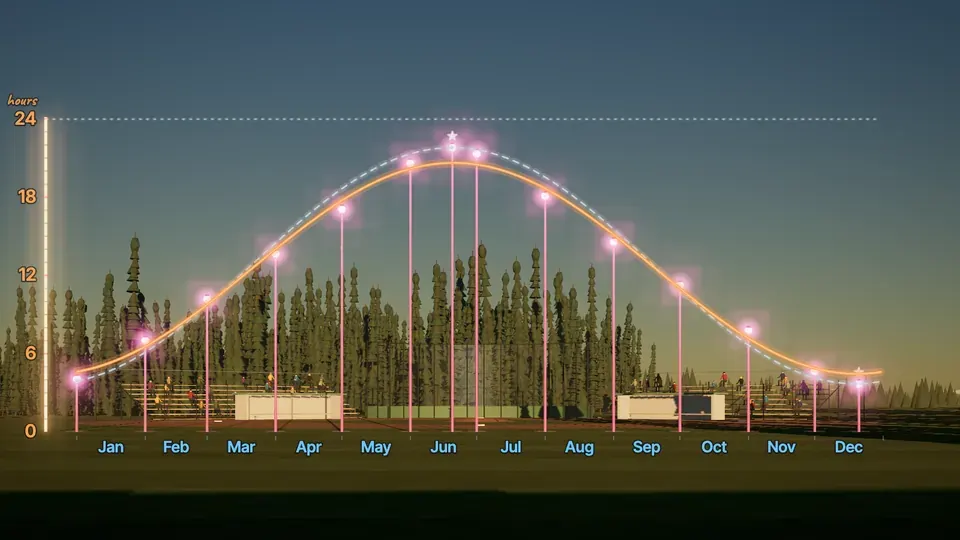
Here’s January first, when the day lasts just four hours and four minutes, so we’ll plant a pole in the outfield that’s exactly that tall on this gauge. Now let’s run the whole year, and on the first of every month we’ll plant another pole, as tall as that day’s daylight. By May the snow is gone, and the days are growing by about three and a half hours a month.

After the end of June the poles start getting shorter, and by December they’re almost back to where they started. Now look at the shape the twelve poles make. They climb, they turn over, they come back down, and next year they’ll do the same thing all over again. A pattern that repeats like that is periodic, and the simplest smooth periodic function we know is a sinusoid, so that’s the shape we’ll fit.

It happens because the Earth’s axis is tilted, so for half of every trip around the Sun, the north leans toward it. But the sinusoid is our guess about the shape, so now we have to make it fit and then test it. Two more readings will help us. The longest day of twenty twenty-five was June twentieth, at twenty-one hours forty-nine minutes, and the shortest was December twenty-first, at three hours forty-two minutes.

Here are all twelve readings. For a formula, the input has to be a number, so t counts the days since January first, which makes January first t equals zero, and May first t equals one hundred twenty.

The output needs care too, because twenty-one hours forty-nine minutes is not twenty-one point four nine. An hour has sixty minutes, so forty-nine minutes is forty-nine sixtieths of an hour, and the longest day is about twenty-one point eight two hours. The same way, the shortest day, three hours forty-two minutes, is exactly three point seven hours, and now every reading is a point on the graph.

Read the wave off the data

A sinusoid needs four numbers, the a, b, c and d from the last lesson, and we can read every one of them off the data. Let’s start with the period. Here’s next year’s data too, and the longest day of twenty twenty-six was June twentieth again, with the same twenty-one hours forty-nine minutes.

From one peak to the next is three hundred sixty-five days, so the period is three hundred sixty-five days, measured in days because t is in days. That gives us the frequency too, because one cycle every three hundred sixty-five days means one three hundred sixty-fifth of a cycle per day. Here’s one for you. The period is three hundred sixty-five days, so which number goes in the model as b?

Now the height of the wave. Let’s put one rail on the longest day and one on the shortest. The whole swing between them is twenty-one point eight two minus three point seven, which is eighteen point one two hours. The amplitude is how far the wave reaches above or below its middle, which is only half the swing, nine point zero six hours.

Eighteen point one two is easy to write down by mistake, but that’s the distance from top to bottom, twice the amplitude. The midline sits exactly halfway between the rails, at their average. Twenty-one point eight two plus three point seven, over two, is twelve point seven six hours.

Now try another city. In Seattle the longest day lasts fifteen hours fifty-nine minutes, and the shortest lasts eight hours twenty-five minutes. What’s the amplitude of a sinusoidal model for Seattle’s daylight?

That’s three of our four numbers, the period, the amplitude and the midline, all read straight off the data. The last one, the shift, is about time, so let’s go back to the field.

Line it up

Here are our poles again, with a cosine strung over them that has our amplitude, our period and our midline. Its height and its swing look right, but look where its peak is. It’s on January first, the darkest time of the year, so this model thinks summer happens in January. A cosine starts at its peak, and we know one real reading that sits right at the top of the year, June twentieth, with twenty-one point eight two hours.

So you line it up. Slide the whole wave along the calendar until its peak sits right on the longest day. Notice what just happened. One real pair of numbers, June twentieth and its twenty-one point eight two hours, decided where the wave sits in time. That’s the shift, and it’s measured in days.

Here’s the whole model. Nine point zero six is the amplitude, two pi over three hundred sixty-five sets the period, minus one hundred seventy moves the peak to day one hundred seventy, and twelve point seven six is the midline. A cosine peaks where the inside is zero, and t minus one hundred seventy is zero when t is one hundred seventy, so even though it’s a minus, it moves the peak to the right. Here c is negative one hundred seventy.

We used cosine because a cosine starts at its peak, and the peak was the date we knew. A sine starts on the midline going up, a quarter of a period before its peak, so with sine the shift is day seventy-eight and three quarters, around March twentieth, the first day of spring. It’s the same wave with a different formula, so on the AP exam, answer in whichever form the question asks for. But a model is only worth something if it works on days it wasn’t built from, so let’s test it.

May first is day one hundred twenty. Switch your calculator to radians first, then find the model’s prediction for May first, to the nearest hundredth of an hour.

The almanac says May first had seventeen hours six minutes, which is seventeen point one hours, so our model is about an hour and a half too generous. It nails the longest day because we built it from that day, but a day it never saw shows the error. Checking a model against real readings is how you find out how good it is.

Let the calculator try

Let’s draw that miss at every one of the twelve readings. Some of the misses are small, but in May and again in August the model is off by about an hour and a half. So why can’t we just fix it? This far north, a year of daylight isn’t exactly a sinusoid. It’s a little pointier at the top, so no sinusoid passes through all of these points.

The best we can do is the sinusoid that misses by the least overall, and that’s exactly what a calculator’s sinusoidal regression finds. It tries the wave in every size and position and keeps the one where the misses, squared and added up, are as small as possible.

We call that least squares, and it’s the same idea behind the regressions you ran in Units One and Two. Here’s the wave it finds. Its amplitude is eight point zero nine, a bit smaller than ours, its midline is twelve point five five, and its peak is at day one hundred seventy point six, half a day after ours.

Its misses are smaller almost everywhere. A typical miss is about half an hour, instead of almost an hour. But look at June twentieth. The regression comes up about seventy minutes short of the longest day, the very day our hand-built model hit exactly.

So neither model is the truth. One is perfect at the peak, and the other is better on average. One more thing. We told the calculator the period, three hundred sixty-five days. Left alone, it would pick about three hundred seventy-four, which shaves off a tiny bit of error, but a year is three hundred sixty-five days, so the context wins.

The twenty-hour days

Back to the ballfield. Here are our twelve poles again, with the regression wave strung over them, and our hand-built wave as a ghost behind it. Now we can answer the question we started with. Let’s put a line across at twenty hours and find the days above it.

So far we’ve used the model to go from a date to the daylight. This time we know the daylight, twenty hours, and we want the date, so we’re going backwards, from an output to an input.

Find the first twenty-hour day. Drag the date marker along the calendar until the regression wave says exactly twenty hours. But there’s a second answer. A sinusoid is symmetric about its peak, and this one peaks at day one hundred seventy point six, twenty-three point four days after the crossing on May twenty-eighth. So the same twenty-three point four days after the peak, it comes back down through twenty hours, on July fourteenth.

Whenever you go backwards on a periodic model, look for the partner, because there’s usually more than one answer. Our hand-built wave makes a very different forecast. It crosses twenty hours on May thirteenth and comes back down on July twenty-seventh, almost a month longer. Two models, two forecasts. When we open the real calendar, which one do you think will be closer?

Here’s the real calendar, every single day of twenty twenty-five, straight from the almanac. The real twenty-hour days run from May twenty-seventh to July fifteenth. The regression said May twenty-eighth to July fourteenth, so from just twelve numbers it landed within a day at each end. And the hand-built model, the one that nailed the longest day, was about two weeks off at each end.

That’s what a good model does. You build it from a handful of real numbers and you test it, and then it tells you something you never measured, like the season of the midnight Sun.

Where a model stops working

Before you trust a model, ask where its data came from. Ours came from one place, Fairbanks, in one year, so its contextual domain is twenty twenty-five, t from zero to three hundred sixty-four. Could we stretch it into twenty twenty-six? With care, yes, because the cycle repeats, and the longest day of twenty twenty-six is June twentieth again, with the same twenty-one hours forty-nine minutes.

But move it north to Utqiagvik, the northernmost town in the United States, where the Sun doesn’t set for about eighty-two days in summer and doesn’t rise for about sixty-four days in winter, so the readings sit flat at twenty-four hours and at zero. Fit a sinusoid to those readings and it can’t sit flat. It bulges up to twenty-four point eight hours in June, which is more daylight than there is day. So a model only works inside its contextual domain, and outside it, it can even give you answers that are impossible.

This is how the exam asks it

On the AP exam, a modeling question often looks like this. A gauge measures a harbor’s water depth every few hours, and you build a sinusoidal model from the readings. The same moves work. The highest readings, ten meters, come at hours two and fourteen, so the period is twelve hours, and b is two pi over twelve, or pi over six.

The highest reading is ten and the lowest is two, so the amplitude is half of eight, four meters, and the midline is the average, six meters. Suppose we only had the first reading, eight meters at time zero. Two waves with these numbers pass through that point. In one the water is rising toward a peak two hours later, and in the other it’s falling from a peak two hours earlier.

At time zero the water is eight meters deep, and it’s rising. Which of these models fits that? That’s exactly how the exam asks it, and it wants you to build the model from the context and say why each number fits the data.

What to remember

The time from one peak to the next is the period, and b is two pi over the period. Half the gap between the highest and lowest readings is the amplitude, and their average is the midline.

A real reading, like the date of a peak, sets the shift, and a different real reading tests the model. Regression finds the wave with the smallest total miss, and either model can predict an output or find the inputs for an output, as long as you stay inside its domain. So the next time you see a game played at midnight in full daylight, you’ll know how to work out, almost to the day, how long that season lasts.